The classical singular value decomposition (SVD) has a long and venerable history. I have described it as a fundamental theorem of linear algebra. Nevertheless, the mathematical property that makes it so useful in general (namely, the orthogonality of the matrix factors) also makes it less useful for certain applications. In response, researchers developed the nonnegative matrix factorization (NMF), which removes the requirement of orthogonality and replaces it with a requirement that the elements in the matrix factors be nonnegative.
The purpose of this article is to use an example to compare the classical singular value decomposition (SVD) and the nonnegative matrix factorization (NMF). An excellent paper that presented the NMF to the statistical community is Fogel, Hawkins, Beecher, Luta, and Young (2013), "A tale of two matrix factorizations." One section of the paper that caught my eye is Section 4.2, "Realistic synthetic mixture," which compares and contrasts the NMF and the classical SVD. This article presents a similar example. It also improves the visualizations in the Fogel et al. paper. The images in this blog post are better for visualizing how the SVD and the NMF methods differ.
Simulating patient-gene data for a disease
The Fogel et al. example is based on clinical study that involves gene expression levels for 30 genes across 40 patient samples. (Actually, the paper uses 40 genes, but the example is more enlightening if the number of variables and observations are different.) Assume a disease (such as diabetes) has two distinct genetic etiologies. The L matrix ("L" for "left side") represents 40 patients. The first column of L represents a measure of one etiology. The second column of L represents a measure of a second etiology. In this example, 10 patients have only the first etiology, 10 have only the second etiology, and 10 have both.
The R matrix ("R" for "right side") represents expression levels for 30 genes. This example assumes the first 10 genes are related to the first etiology, and the next 10 genes are related to the second etiology. The last 10 genes are not related to the disease.
You can use SAS IML to simulate these factors and to construct the data matrix as their product. Because the data are simulated, we know that the data matrix is exactly rank-2, and we know a true set of rank-2 matrices whose product equals the data matrix. You can simulate the L and R matrices by randomly assigning a value between 1 and 2 to specific cells. Notice that these factors are entirely nonnegative, so the product matrix, X = L*R, is also nonnegative. The following SAS IML statements simulate the L and R matrices and create heat maps to visualize them.
proc iml; reset fuzz; /*** Simulation of L and R for clinical example of two etiologies ***/ call randseed(123); nrow = 40; ncol = 30; L = j(nrow, 2, 0); idx1 = (11:20) || (31:40); L[idx1, 1] = randfun( ncol(idx1), "Uniform", 1, 2); /* 1st col */ idx2 = 21:40; L[idx2, 2] = randfun( ncol(idx2), "Uniform", 1, 2); /* 2nd col */ R = j(2, ncol, 0); idx1 = 1:10; R[1, idx1] = randfun( 1|| ncol(idx1), "Uniform", 1, 2); /* 1st row */ idx2 = 11:20; R[2, idx2] = randfun( 1||ncol(idx2), "Uniform", 1, 2); /* 2nd row */ /* simplify L and R by rounding to 2 decimal places */ L = round(L, 0.01); R = round(R, 0.01); /*** end simulation of L and R ***/ /* create blue-white-red color ramp from ColorBrewer */ %let BlueReds = CX2166AC CX4393C3 CX92C5DE CXD1E5F0 CXF7F7F7 CXFDDBC7 CXF4A582 CXD6604D CXB2182B ; %let Reds = CXF7F7F7 CXFDDBC7 CXF4A582 CXD6604D CXB2182B ; /* Visualize L (40 rows, transposed for viewing) and R (30 columns) */ ods graphics / width=640px height=84px; call heatmapcont(L`) colorramp={&BlueReds} yvalues={'Real 1' 'Real 2'} range={-2.2 2.2} title="Original L`"; ods graphics / width=480px height=84px; call heatmapcont(R) colorramp={&BlueReds} yvalues={'Real 1' 'Real 2'} range={-2.2 2.2} title="Original R"; |
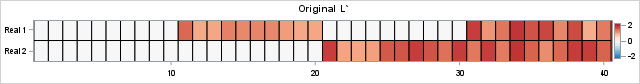
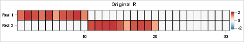
The columns of the L matrix are the factors for gene activation. The rows of the L matrix represent patients. (Note: the image is for the transposed matrix, L`). You can visualize the etiologies for the four groups. For the R matrix, the rows are the factors and the columns are the genes. The heat maps are entirely red or white because all values of L and R are nonnegative. The product, X = L*R, represents the gene expression levels for 30 genes across 40 patient samples. The following statements visualize the data matrix:
X = L*R; ods graphics / width=360px height=480px; /* Note: Dark red now represents 4, not 2.2 */ call heatmapcont(X) colorramp={&Reds} range={-0.01 4.04} title="Original (Synthetic) Data Matrix"; |
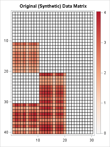
In the real world, the order of the patients and the order of the genes would be permuted arbitrarily. Also, there would be random noise that appears in the 40x30 panel of measurements. Regardless, when presented with these data, a researcher would like to recover the underlying factors that generated them. If researchers know or suspect that the disease has two etiologies, they might try to approximate the matrix by using a rank-2 decomposition of factors. In this example, we know the true factors whose product forms the X matrix, but in the real world, those factors are unknown and must be estimated from X.
The SVD factorization
The classical way to decompose X into rank-2 factors is to use the singular value decomposition (SVD). A newer decomposition is the nonnegative matrix factorization (NMF). Following Fogel et al. (2013), the remainder of this article compares these two factorizations.
A previous article discusses the fact that a low-rank factorization is not unique, but can be arbitrarily rescaled and permuted. Fogel et al. visualized the results by using heat maps. However, their heat maps are individually scaled to use the minimum and maximum value in each matrix. Because the SVD factors have positive and negative elements whereas the NMF factors do not, it is hard to compare the two factorization methods unless the colors in the heat maps represent the same scale. In this article, I carefully scale the factors so that red colors always represent positive values, white represents zero, and blue always represents negative values.
Let's look at an SVD analysis of the simulated data matrix, X. The following statements call the SVD subroutine in SAS IML to compute X = U*D*V`. To get the rank-2 approximation of X, the first two columns of U and V are extracted. For this example, the rank-2 product exactly equals X because we constructed X as the product of two rank-2 matrices and did not add any noise.
k = 2; call SVD(A, D, B, X); i = 1:k; L_SVD = A[, i] # sqrt(D[i])`; /* scale each factor evenly */ R_SVD = T(B[, i] # sqrt(D[i])`); X2 = L_SVD*R_SVD; /* show that the SVD recovers X exactly */ maxDiff = max(abs(X-X2)); print maxDiff; |

Interpreting the SVD factors
Although the product of the SVD exactly equals X, the SVD factors do NOT look like the nonnegative factors L and R that were used to create X. The reason is that the factors in an SVD are orthogonal, which means that the factors must contain both positive and negative elements when k ≥ 2. (Technically, if X is block-diagonal, then the SVD can recover the original features, but that is not the case in this example.) Because X contains strictly nonnegative values and isn't block-diagonal, it is mathematically impossible for the SVD to return orthogonal factors that are entirely nonnegative.
This fact is shown by using the following heat maps, which display the SVD factors on the same color scale as the true factors.
/* Visualize true L` (40 columns) and the left factor from the SVD */ ods graphics / width=640px height=84px; call heatmapcont(L`) colorramp={&BlueReds} yvalues={'Real 1' 'Real 2'} range={-2.2 2.2} title="Real Factor L`"; call heatmapcont(L_SVD`) colorramp={&BlueReds} yvalues={'SVD 1' 'SVD 2'} range={-2.2 2.2} title="SVD Factor"; |
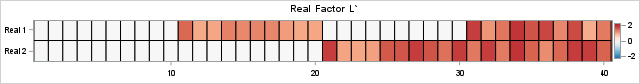
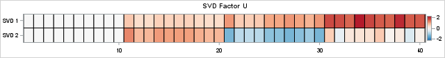
The heat maps show (the transpose of) the original factor, L, and the SVD factor, U. Whereas the true factors for X have strictly nonnegative values, the second factor in the SVD contains negative values (the blue cells). The negative values are required because of orthogonality: the inner product of the columns must equal 0! The negative values represent contrasts, which can be difficult to interpret when the true underlying components of the data are strictly additive.
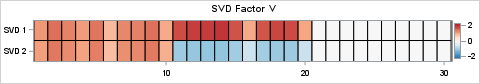
You can use similar statement to visualize the right-hand SVD factor, V, and compare it to the original factor, R. The results are shown below:

The NMF factorization
The SVD cannot return purely nonnegative factors, which makes interpretation of the factors difficult when the data are nonnegative. Researchers developed the NMF to address this issue. The NMF decomposes a nonnegative matrix into a product W*H, where the elements in W and H are constrained to be nonnegative. The decomposition is not unique.
Let's use NMF to produce rank-2 factors of X. In SAS, you can obtain the NMF by using PROC NMF in SAS Viya, or by implementing the algorithm directly in SAS IML. This article computes the NMF by running an IML module that implements the Lee and Seung multiplicative update algorithm. The factorization you get might depend on the way that you specify an "initial guess" for the factors. Consequently, the result that I present is just one possible NMF factorization.
The NMF returns two rank-2 matrices, W and H, such that X ≈ W * H. As with the SVD, the product is a rank-2 approximation to X. However, due to the algorithm and initialization that I used, the product of the NMF factors does not exactly equal X. The NMF algorithm attempts to optimize a non-convex objective function. It can converge to local minima.
/* Run the Lee and Seung "multiplicative update" algorithm for NMF. The IML implementation can be downloaded from GitHub. */ run nmf_mult(W1, H1, X, 2); /* Let's see whether the product W1*H1 is a reasonable approximation of X. */ X_est = W1*H1; ods graphics / width=360px height=480px; /* Note: Dark red now represents ~4, not 2.2 */ call heatmapcont(X_est) colorramp={&Reds} range={-0.01 4.04} title="NMF Estimate of Matrix"; |
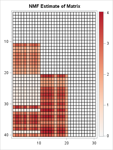
According to the heat map, the product W1*H1 does a very good job approximating X. An obvious difference is seen for Patients 32 and 39. Whereas these patients actually have positive gene expression levels for genes 1-10, the rank-2 NMF approximation does not fully recover that fact.
Comparing the NMF factors
As explained in the previous article, there are two inherent ambiguities in the factors of the NMF:
- The columns of W and the rows of H can be arbitrarily scaled, provided they are scaled reciprocally.
- The columns of W and the rows of H can be arbitrarily permuted, provided they are permuted together.
To compare the factors from the NMF with the original factors, it is best that the colors represent the same scale. We could standardize the factors L and R, but since we have already visualized them, I will instead adjust the scaling of W and H so that their maximum elements are approximately equal to 2, which was the maximum value in the original L and R factors. This is not a standard way to standardize (pun intended!), but it is useful for this example.
/* The following statements rescale W and H to try to put all values in [0,2]. */ maxVal = 2; scale = maxVal / W1[<>,]; /* scale each col by maximum, then multiply by maxVal */ W = W1 # scale; /* scale columns of W */ H = H1 / scale`; /* reciprocally scale rows of H */ /* Now, visualize the NMF factors, W and H, and compare with L and R from the original simulation. */ ods graphics / width=640px height=70px; call heatmapcont(L`) colorramp={&BlueReds} yvalues={'Real 1' 'Real 2'} range={-2.2 2.2} title="Real Factor L`"; call heatmapcont(W`) colorramp={&BlueReds} yvalues={'NMF 1' 'NMF 2'} range={-2.2 2.2} title="NMF Factor W`"; |
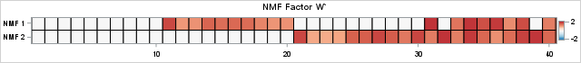
For some data, you might need to permute the columns of the left NMF factor and the rows of the right factor before you can compare them to real factors. (An easy way to compare: sort the columns of all left factors from largest to smallest by using the Euclidean norm.) In this example, we got lucky and can immediately compare the NMF and real factors. The similarity between the left factors is impressive. The NMF factor captures the structure of the real factor except for Patients 32 and 39. In this case, the NMF algorithm converged to a solution that is not the true factor. This happens frequently. One of the drawbacks of NMF is that the solution you get depend on an initial guess for the factors, and there are many competing ideas about how to provide an initial guess.
The agreement between the right factors is also impressive, as shown below:
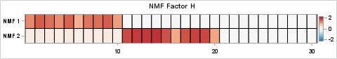
This output highlights two critical features of the NMF algorithm:
- Both factors contain only nonnegative elements. It immediately follows that the product W*H must also be nonnegative.
- The NMF decomposition does an excellent job of recovering the true underlying factors. If you compare the true factors with the NMF factors, you can see that the patterns are remarkably similar. The most obvious difference is that the first row of the transposed W factor does not correctly estimate the values for Patients 32 and 39. The NMF estimate indicates that these patients only exhibit the second etiology, whereas in reality, they exhibit both.
Summary
This article uses SAS IML to present an example that is similar to Section 4.2 in Fogel, et al. (2013). The example simulates a data matrix that represents the expression profiles of 30 target genes for 40 clinical study participants. A classical SVD analysis produces factors whose product perfectly equals X. The SVD uses deterministic linear algebra, and is guaranteed to find an optimal rank-k approximation. However, the factors contain both positive and negative values because the SVD enforces orthogonality of the factors.
In contrast, the NMF produces factors that contain strictly nonnegative values. When the true underlying features of the data involve positive quantities whose effects are additive, the NMF factors are more natural and interpretable. However, the NMF attempts to optimize a non-convex objective function. The algorithm's solution depends on how the algorithm is initialized. Some results might correspond to local minimum instead of a global one.

1 Comment
Pingback: On the nonuniqueness of low-rank matrix factors - The DO Loop