SAS supports more than 25 common probability distributions for the PDF, CDF, QUANTILE, and RAND functions. If you need a less-common distribution, you can implement new distributions by using Base SAS (specifically, PROC FCMP) or the SAS/IML language. This article shows how to use call functions related to the three-parameter Burr XII distribution, which is also known as the Singh-Maddala distribution in econometrics. If you have a license for SAS/ETS software, you already have access to these functions, as shown in Appendix 2. If you do not have a license for SAS/ETS, this article shows how to implement them in PROC FCMP in Base SAS.
What is the Burr XII distribution?
The Burr distribution is a flexible distribution. It is used to model skewed positive data such as household income. In shape, it is similar to the Lognormal, Gamma, and Weibull distributions, but the Burr distribution can model data that has large kurtosis relative to the skewness. The tail of the Burr distribution drops off like a power law instead of decaying exponentially.
Some density functions are shown to the right for three sets of parameter values. This article uses the same parameter names as PROC SEVERITY in SAS/ETS software:
- The scale parameter is Theta (or θ in formulas). The Wikipedia article about the Burr distribution uses λ for the scale parameter.
- The first shape parameter is Alpha (α). The Wikipedia article uses k for the first shape parameter.
- The second shape parameter is Gamma (γ). The Wikipedia article uses c for the second shape parameter.
The shape parameters determine the shape of the distribution. For household income data in the US and Europe, Alpha (k) might have values in the range[1, 3] and Gamma (c) might have values in [1.5, 2.5]. For models of insurance claims, Alpha (k) might be ~0.5 whereas Gamma (c) might be in the range [15, 20].
The following list shows the mathematical formulas for the PDF, CDF, and quantile functions for the Burr XII distribution:
- PDF: \(f(x; \theta, \alpha, \gamma) = \frac{\alpha \gamma}{\theta} \left( \frac{x}{\theta} \right)^{\gamma - 1} \left[ 1 + \left( \frac{x}{\theta} \right)^{\gamma} \right]^{-(\alpha + 1)} \quad \text{for } x > 0\)
- CDF: \(F(x; \theta, \alpha, \gamma) = 1 - \left[ 1 + \left( \frac{x}{\theta} \right)^{\gamma} \right]^{-\alpha} \quad \text{for } x > 0\)
- Quantile function: \(Q(p; \theta, \alpha, \gamma) = \theta \left( (1 - p)^{-\frac{1}{\alpha}} - 1 \right)^{\frac{1}{\gamma}} \quad \text{for } 0 < p < 1\)
Define the Burr functions in PROC FCMP
This article defines the four main functions that statistical programmers need: The PDF, CDF, quantile, and random functions. They are defined in a PROC FCMP library and can be called from the SAS DATA step. The library also contains the log-PDF function, which is important for using MLE to fit parameters of the model to data.
To simplify the article, I've put the PROC FCMP code in Appendix 1. To reproduce the images in this article, be sure to run the PROC FCMP code before running the examples. You must also execute the following SAS statement before calling the functions in the DATA step:
options cmplib=work.funcs; /* define location of Burr functions so the DATA step can find them */ |
Parameter values for the examples
In three-parameter families, it can be difficult to visualize all possible shapes. In these examples, I set the scale parameter (Theta) to 1 because the scale parameter does not change the shape of the distribution. In the original paper by Burr (1942), he used Gamma ≥ 1 and Alpha ≥ 1. In addition, Rodriguez (Biometrika, 1977) points out the that Burr distribution has finite kurtosis only when (Gamma ⋅ Alpha) ≥ 4. This article shows two examples where (Gamma ⋅ Alpha) ≥ 4 and one example that does not have finite skewness or kurtosis.
The following macro definitions make it easier to use the same parameter values for all examples.
- The %DefineParms macro defines three parameter values. I set the scale parameter to 1 because it does not affect the shape.
- The %DefineGroup macro defines two ID variables: ID and Group. The ID variable contains the numbers 1-3. The Group variable defines a character string that contains the parameter values.
- The MaxX macro truncates the graphs so that the data range is [0,4], which is sufficient for these parameter values. Since the Burr distribution has a heavy tail, random samples from the Burr distribution might contain extreme values.
/* Theta : Scale > 0 (this is "lambda" in Wikipedia) Alpha : Shape1 > 0 (this is "k" in Wikipedia) Gamma : Shape2 > 0 (this is "c" in Wikipedia) */ %macro DefineParms; array Theta[3] _temporary_ (1, 1, 1); array Alpha[3] _temporary_ (2, 0.5, 3); /* k */ array Gamma[3] _temporary_ (1, 10, 2); /* c */ %mend; %macro DefineGroup; length Group $40; ID = i; Group = cats("Theta=",put(Theta[i],BEST3.), ", Alpha=",put(Alpha[i],BEST3.), ", Gamma=",put(Gamma[i],BEST3.) ); %mend; %let MaxX = 4; /* for visualization, truncate data range (0, MaxX] */ |
The Burr PDF
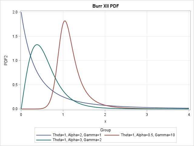
When I study a new distribution, I always start by visualizing the probability density function (PDF). The visualization enables you to recognize the shapes of data distributions that can be modeled by the distribution. The following DATA step calls the PDF_Burr function (see the instructions in the section, "Define the Burr functions in PROC FCMP"), then uses PROC SGPLOT to visualize the PDF curves:
data PDF_Test; %DefineParms; dx = 0.025; do i = 1 to dim(Theta); %DefineGroup; do x = constant('MACEPS'), dx to &MaxX by dx; PDF = PDF_Burr(x, Theta[i], Alpha[i], Gamma[i]); output; end; end; keep x PDF ID Group; run; title "Burr XII PDF"; proc sgplot data=PDF_Test; series x=x y=PDF / group=Group lineattrs=(thickness=2); yaxis grid; xaxis grid; run; |
The graph is shown at the top of this article. You can see that the blue curve (Alpha=2, Gamma=1) has a mode at x=0. It has a negative slope at x=0 and rapidly decreases. The red curve (Alpha=0.5, Gamma=10) has a mode near x=1; the slope at x=0 is close to 0. The green curve (Alpha=3, Gamma=2) has a mode near x=1; the slope at x=0 is positive.
The Burr CDF
The cumulative distribution function (CDF) is the integral of the PDF. Given a value, x, the CDF at x tells you the probability that a random observation drawn from the Burr distribution will be less than x. The following DATA step calls the CDF_Burr function, then uses PROC SGPLOT to visualize the CDF curves:
data CDF_Test; %DefineParms; dx = 0.025; do i = 1 to dim(Theta); %DefineGroup; do x = constant('MACEPS'), dx to &MaxX by dx; CDF = CDF_Burr(x, Theta[i], Alpha[i], Gamma[i]); output; end; end; keep x CDF ID Group; run; title "Burr XII CDF"; proc sgplot data=CDF_Test; series x=x y=CDF / group=Group lineattrs=(thickness=2); yaxis grid min=0 max=1; xaxis grid; run; |
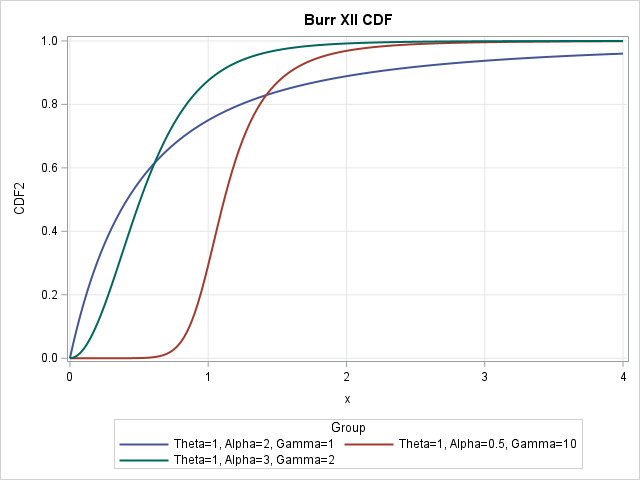
For any value of x along the horizontal axis, the graph shows the probability (on the vertical axis) that a random observation is less than x. For example, the red curve at x=1 shows that there is approximately a 30% chance that a random variate from that distribution will have a value less than 1.
The Burr quantile function
The quantile function is the inverse of the CDF function. Given a probability, p in (0,1), the quantile function at p is the x value such that a random observation drawn from the Burr distribution will be less than x with probability p. For the Burr distribution, you can explicitly solve the equation CDF(x) = p for p as a function of x. The following DATA step calls the Quantile_Burr function, then uses PROC SGPLOT to visualize the quantile curves. The graph is not shown because it is simply a flipped version of the CDF graph:
data Quantile_Test; %DefineParms; dp = 0.005; do i = 1 to dim(Theta); %DefineGroup; do p = constant('MACEPS'), dp to 1-dp by dp; x = Quantile_Burr(p, Theta[i], Alpha[i], Gamma[i]); output; end; end; keep p x ID Group; run; title "Quantiles for Burr XII"; proc sgplot data=Quantile_Test; series x=p y=x / group=Group lineattrs=(thickness=2); yaxis grid min=0 max=&MaxX; run; |
Random variates from the Burr distribution
You can use the quantile function to generate random variates from the Burr distribution. This is called the "inverse CDF method" for simulating data. The following DATA step calls the Rand_Burr function, which generates a random uniform value in (0,1) and then calls the Quantile_Burr function. Whereas the other functions were visualized by overlaying curves on a single plot, it is easier to see the distribution of the random variates if you call SGPANEL to create a panel that has three histograms. The Burr distribution can generate very large extreme values. The call to PROC SGPLOT uses a WHERE clause to exclude large values so that the scale of the histograms is the same as the scale of the graphs in the previous sections.
data Rand_Test; call streaminit(1234); %DefineParms; N = 1000; do i = 1 to dim(Theta); %DefineGroup; do j = 1 to N; x = Rand_Burr(Theta[i], Alpha[i], Gamma[i]); output; end; end; keep x ID Group; run; title "Burr Random Variates"; proc sgpanel data=Rand_Test; WHERE x <=&MaxX; /* OPTIONAL: Truncate the extreme values */ panelby Group / columns=1 novarname; histogram x; run; |
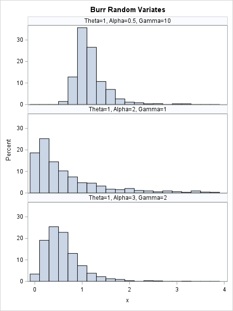
Because the program generates 1,000 random variates, the shapes of the histograms (truncated to (0,4]) are similar to the shapes of the PDF curves.
Summary
The Burr XII distribution is used in economics. If you have a license for the SAS/ETS product, you already have access to built-in functions (with different names) for the Burr distribution. (See Appendix 2 for the syntax.) For SAS customers who do not license SAS/ETS, this article shows how to define four related functions in PROC FCMP in Base SAS: the PDF, CDF, quantile, and random variate functions. The definitions are based on an old SAS/ETS example and use the same names for the parameters as PROC SEVERITY.
In a future article, I will show how to use SAS to fit the parameters of the Burr distribution to data.
Appendix 1: Define FCMP functions for the Burr distribution
This appendix shows how to use PROC FCMP in SAS to add new DATA step functions. It follows the same technique as a previous article about the generalized extreme-value (GEV) distribution. Run this PROC FCMP step before trying to call the functions in the DATA step.
/* Define the PDF, log-PDF, CDF, and QUANTILES of the Burr XII distribution in PROC FCMP. These formulas use the same parameter names as PROC SEVERITY is SAS/ETS software. The library is based on code at https://support.sas.com/documentation/onlinedoc/ets/ex_code/151/svrtBurr.html The SAS/ETS product includes built-in functions (with different names) that you can call. The support for the Burr distribution in x > 0. The Burr distribution has three parameters: Theta : Scale > 0 (this is "lambda" in Wikipedia) Alpha : Shape1 > 0 (this is "k" in Wikipedia) Gamma : Shape2 > 0 (this is "c" in Wikipedia) */ proc fcmp outlib=work.funcs.ProbDist; function PDF_Burr(x, Theta, Alpha, Gamma); if x < constant('MACEPS') then return (0); T1 = Gamma*Alpha/Theta; z = x / Theta; T2 = z**(Gamma-1); T3 = (1+z**Gamma)**(-Alpha-1); return( T1*T2*T3 ); endsub; function LOGPDF_Burr(x, Theta, Alpha, Gamma); if x < constant('MACEPS') then return (.); z = x/Theta; L1 = log(Gamma*Alpha/Theta); /* log(c*k/lambda) */ L2 = (Gamma-1)*log(z); /* log(x^{Gamma-1}) */ L3 = -(Alpha+1) * log1px(z**Gamma); /* log(1+x^c)^{-k-1} */ return( L1 + L2 + L3 ); endsub; function CDF_Burr(x, Theta, Alpha, Gamma); if x < constant('MACEPS') then return (0); z = x/Theta; return( 1 - (1 + z**Gamma)**(-Alpha) ); endsub; function Quantile_Burr(p, Theta, Alpha, Gamma); if p < constant('MACEPS') | p > 1-1.0e-14 then return (.); D = (1-p)**(-1/Alpha); return( Theta * (D - 1)**(1/Gamma) ); endsub; function Rand_Burr(Theta, Alpha, Gamma); p = rand("Uniform"); x = Quantile_Burr(p, Theta, Alpha, Gamma); return (x); endsub; quit; options cmplib=work.funcs; /* define location of Burr functions so the DATA step can find them */ |
Appendix 2: Call built-in SAS/ETS functions
If you have a license for the SAS/ETS product, you can call the following built-in functions: Burr_PDF, Burr_LogPDF, Burr_CDF, and Burr_Quantile. The underlying formulas are the same as in this article.
options cmplib=Sashelp.Svrtdist; /* functions are in SASHELP */ %let MaxX = 4; /* for visualization, truncate data range (0, MaxX] */ data ETS_Calls; call streaminit(1234); Theta = 1; Alpha = 0.5; Gamma = 10; dx = 0.025; do x = constant('MACEPS'), dx to &MaxX by dx; PDF = Burr_PDF(x, Theta, Alpha, Gamma); logPDF = Burr_logPDF(x, Theta, Alpha, Gamma); CDF = Burr_CDF(x, Theta, Alpha, Gamma); Qntl = Burr_Quantile(CDF, Theta, Alpha, Gamma); /* there isn't a pre-defined Burr_Rand function */ u = rand("Uniform"); y = Burr_Quantile(CDF, Theta, Alpha, Gamma); /* random from Burr */ output; end; run; |
