I write a lot of Monte Carlo simulations. This article discusses how to assess whether two independent Monte Carlo estimates are close to each other. This result can be used to test the correctness of a Monte Carlo simulation. It can also be used to compare different Monte Carlo algorithms that compute the same quantity.

A Monte Carlo (MC) simulation provides both a statistical estimate for a parameter and a confidence interval for the parameter. (The confidence interval assumes that the estimate follows a normal distribution.) If you run two independent MC simulations to estimate the same parameter, how close will the two estimates be? This is illustrated by the diagram to the right. There are two MC estimates (q1 and q2) and two confidence intervals for an unknown parameter, μ. How close are the estimates to each other? Intuitively, you might expect to bound the distance between the estimates by the width of the larger confidence interval, but is there a better way to compare the distance between two estimates?
Yes, there is a better way. You can compute the variance of the difference between the two estimates and construct a 95% confidence interval for that difference. This article shows how to perform the computation in SAS by using the SAS IML language. We will also verify the empirical 95% coverage for an example.
Generate independent Monte Carlo estimates
To make the ideas concrete, let's look at a specific problem. Suppose you want to estimate the expected value of the Exponential distribution with scale parameter 10. Call that quantity μ. You can prove analytically that μ = 10 is the true expected value.
The following SAS IML function performs a Monte Carlo simulation to estimate μ. The function generates B independent samples of size N from the Expo(10) distribution. It calculates the mean of each sample. The Monte Carlo estimate is the average of the estimates. The Monte Carlo standard error is the standard deviation of the estimates divided by sqrt(B).
proc iml; /* use Monte Carlo simulation to estimate the mean of the Expo(lambda) distribution. The simulation uses B independent samples of size N. Each sample is independently drawn from Expo(lambda) */ start MC_Est_Expo(N, B, lambda); x = j(N, B, .); call randgen(x, "Expo", lambda); sample_means = mean(x); /* mean of each column */ MC_est = mean(sample_means`); /* MC estimate of statistic */ SE_est = std(sample_means`) / sqrt(B); /* MC standard error */ return( MC_est || SE_est ); finish; N = 100; B = 5000; lambda = 10; call randseed(79); est1 = MC_Est_Expo(N, B, Lambda); est2 = MC_Est_Expo(N, B, Lambda); print est1[c={'MCest1' 'SE1'}], est2[c={'MCest2' 'SE2'}]; |
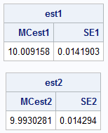
Because the algorithm relies on random number simulation, every call results in a slightly different point estimate and standard error. Here, the estimate from the first simulation is larger than the true parameter (10); the other estimate is smaller. The standard errors are very similar: approximately 0.142.
The variance of the difference
Let q1 and q2 be two independent MC estimates, with standard errors SE1 and SE2. Since both estimates are computed by the same method, the expected value of their difference is zero: E[q1 - q2] = 0. (If we used different methods, and those methods are biased by different amounts, the expected value will not be zero.)
How much variance should we expect for the difference? Because q1 and q2 are independent, the variance of their difference is the sum of the individual variances:
Var(q1 - q2) = SE12 + SE22
Let SEdiff be the square root of this sum. For this example, both estimates are normally distributed, so the difference also follows a normal distribution: q1 - q2 ∼ N(0, SEdiff). You can use this distribution to construct a 95% interval for the difference. Let's do that, then check whether the distance between these estimates |q1 - q2| is less than the width of the interval.
/* given (q1, SE1) and (q2, SE2), what is a confidence interval for the difference q1-q2? The expected value E[q1-q2] = 0, but what is the variance? */ q1 = est1[1]; q2 = est2[1]; SE1 = est1[2]; SE2 = est2[2]; /* Standard deviation of the DIFFERENCE between two independent estimates */ SE_diff = sqrt(SE1**2 + SE2**2); print SE1 SE2 SE_diff; /* Can we bound |q1 - q2| with high probability? Use a prediction interval based on the fact that q1-q2 ~ N(0, SE_diff) */ w95 = quantile("Normal", 0.975) * SE_diff; if abs(q1 - q2) < w95 then print "The difference |q1 - q2| is inside a 95% confidence interval"; else print "The difference |q1 - q2| is NOT inside a 95% confidence interval"; |
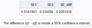
For these estimates, the difference is, indeed, less than the width of a 95% confidence interval. Of course, we might have gotten lucky. The next section investigates what happens if we repeat this experiment many times.
Verify the empirical coverage
According to probability theory, the difference between the two estimates should fall inside the calculated interval 95% of the time. However, I always like to verify statistical theory by running a simulation in SAS.
The following program repeats the experiment 1,000 times. For each iteration, the program generates two independent Monte Carlo estimates, computes the 95% confidence interval for their difference, and saves a 0/1 binary value that indicates if the difference falls inside the CI.
/* If we repeat this computation many times, about 95% of the differences should be in the 95% CI */ C = 1000; crit_val = quantile("Normal", 0.975); /* ~ 1.96 */ inCI95 = j(C, 1, 0); do i=1 to C; est1 = MC_Est_Expo(N, B, Lambda); est2 = MC_Est_Expo(N, B, Lambda); q1 = est1[1]; q2 = est2[1]; SE1 = est1[2]; SE2 = est2[2]; SE_diff = sqrt( (SE1**2 + SE2**2) ); w95 = crit_val * SE_diff; inCI95[i] = (abs(q1 - q2) < w95); end; propInCI = mean(inCI95); print propInCI[c={'Empirical 95% Cov'}]; |
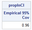
Ah, success! The empirical coverage for this random number seed is close to the theoretical coverage of 0.95. This confirms that adding the individual variances provides a statistical interval for comparing the distance between two Monte Carlo estimates of the same quantity.
Modifying this technique
You can change the critical value if you want to test the difference with more confidence. For example, you can use three standard errors to obtain a 99.7% confidence interval, which is known as the "three-sigma rule."
You can also compare the distance between two estimates that come from different (unbiased) estimates. For example, if one estimate is computed by using B1=5,000 random samples and the other is computed by using B2=3,000 random samples, the standard error for the second estimate will be larger, but you can still compute the standard error of the difference.
If you are testing a routine that produces a random or quasi-random result, you can use this technique to compare the routine's result to a MC validation procedure that you wrote yourself. Suppose the routine returns the value q1. Your validation procedure gives the value q2. 95% of the time, q1 will be close to q2. But there is a 5% chance that they are not sufficiently close. Does that indicate that the estimates are wrong? No, most likely you got unlucky. One option is to rerun the routine and your verification procedure again. This gives new estimates q3 and q4. These new results also have a 5% chance of failure, but the probability that BOTH tests fail sequentially is a very small 0.25%. If that probability is not small enough for you, you can use 99.7% CIs instead of 95% CIs.
Summary
This article shows a technique for comparing the difference between two Monte Carlo estimates of the same quantity. You can compute the variance of the difference as the sum of the two individual variances. In many cases, the expected value of the difference is zero, and the difference is normally distributed. (You should check this assumption.) Therefore, you can derive a formula for the magnitude of the difference. You can use this formula to verify the consistency of a single Monte Carlo simulation, or you can use it to verify that two different MC algorithms provide consistent estimates of the same quantity.