SAS has more than 25 common probability distributions that are supported in the PDF, CDF, QUANTILE, and RAND functions. If you want to work with a less common distribution, you can implement these functions yourself. For example, I previously showed how to use PROC FCMP in Base SAS to implement the Burr (Type XII) distribution and the generalized extreme value distribution.

A SAS programmer recently asked me questions about a zero-inflated (ZI) probability distribution. Some readers might be familiar with distributions that are related to zero-inflated counts. These distributions are used in some linear regression models. A zero-inflated model is a mixture of two distributions: a discrete probability mass situated at X=0, and a second probability distribution, which describes the probability that a random variable is not zero. In regression, two common zero-inflated distributions are the ZI Poisson (ZIP) and the ZI negative binomial (ZINB) distributions.
However, the SAS programmer wanted to implement a mixture distribution that is the mixture of a discrete point-mass distribution and a continuous distribution. The discrete distribution gives the probability that X=0. The continuous distribution gives the probability that X > 0.
This article shows how to use SAS to create functions for the zero-inflated Beta distribution. The image to the right shows the PDF for a ZI Beta distribution. The techniques in this article can be generalized to other mixture distributions, such as a ZI gamma distribution. This article implements the functions in PROC FCMP and calls them from the DATA step.
What is the zero-inflated Beta distribution?
The Beta distribution is a two-parameter distribution on the interval (0,1). The two positive shape parameters are often called "alpha" and "beta." To reduce confusion, I capitalize the name of the distribution and lowercase the name of the parameter. Depending on the relative magnitudes of the shape parameters, the probability density function can be U-shaped, J-shaped, L-shaped, or mound-shaped (sometimes called "inverted-U shaped").
The equation for the probability density function (PDF) of a random variable that follows a zero-inflated distribution is
f(x) = π δ(x) + (1-π) f2(x; α, β) I(x > 0)
where δ(x) is the Dirac delta function, π is the mixing probability, f2 is the probability density function of the second distribution, and I is the indicator function (also called the Heaviside function). For this article, f2 is the PDF of a Beta distribution.
This article uses the values α = 2 and β = 3 for the shape parameters. For the probability of mixing, this article uses π = 0.2. In programs, I use the variable p0 instead of π for the mixing probability so that the parameter will not be confused with the mathematical constant 3.14159....
Define the zero-inflated functions in PROC FCMP
This article defines the four main functions that statistical programmers need: The PDF, CDF, quantile, and random functions for the ZI Beta distribution. They are defined in a PROC FCMP library and can be called from the SAS DATA step. To simplify the article, I've put the PROC FCMP code in the Appendix. To reproduce the images in this article, you must run the PROC FCMP code before running the examples! I have stored the definitions in the WORK libref, but you replace WORK with a libref to a permanent location if you want to persist the definitions. If you do, be sure to specify the CMPLIB= option in each new session of SAS. The CMPLIB= option tells SAS where you stored the functions.
Parameter values for the examples
To keep this article short, all examples use the same parameter values for the Beta distribution. The %DefineParms macro defines three parameter values. It sets the mixing probability (p0) to 0.2. It sets the Beta parameters to α = 2 and β = 3. You can modify the macro to explore other ZI Beta shapes.
%macro DefineParms; p0 = 0.2; alpha = 2; beta = 3; length Params $40; Params = cats("alpha=",put(alpha,BEST3.), ", beta=", put(beta,BEST3.)); %mend; |
The ZI Beta PDF
When I study a new distribution, I start by visualizing the probability density function (PDF). The following DATA step calls the PDF_ZIBeta function, then uses PROC SGPLOT to visualize the PDF curves. Remember to run the code in the Appendix first!
data PDF_Test; %DefineParms; dx = 0.01; do x = 1E-6, dx/2, dx to 1 by dx; PDF = PDF_ZIBeta(x, p0, alpha, beta); output; end; t = 0; output; keep p0 x PDF Params t; run; title "PDF of Zero-Inflated Beta"; proc sgplot data=PDF_Test; series x=x y=PDF / group=Params lineattrs=(thickness=2); dropline x=t y=p0 / dropto=x lineattrs=GraphData1(thickness=5); yaxis grid min=0 offsetmin=0; xaxis grid; run; |
The graph is shown at the top of this article. I used a DROPLINE statement to display a vertical bar, which indicates the discrete probability mass at x=0. The Beta curve defines the probability density for x > 0.
The ZI Beta CDF
The cumulative distribution function (CDF) is the integral of the PDF. Given a value, x, the CDF at x tells you the probability that a random observation drawn from the ZI Beta distribution will be less than or equal to x. Because of the point-mass at 0, the CDF for the ZI Beta distribution has the value p0 (here, 0.2) at x=0 and increases monotonically as x increases. The following DATA step calls the CDF_ZIBeta function, then uses PROC SGPLOT to visualize the CDF curves:
data CDF_Test; %DefineParms; dx = 0.01; do x = 1E-6, dx/2, dx to 1 by dx; CDF = CDF_ZIBeta(x, p0, alpha, beta); output; end; t = 0; output; keep p0 x CDF Params t; run; title "CDF of Zero-Inflated Beta"; proc sgplot data=CDF_Test; series x=x y=CDF / group=Params lineattrs=(thickness=2); dropline x=t y=p0 / dropto=x lineattrs=GraphData1(thickness=2); yaxis grid min=0 offsetmin=0; xaxis grid; run; |
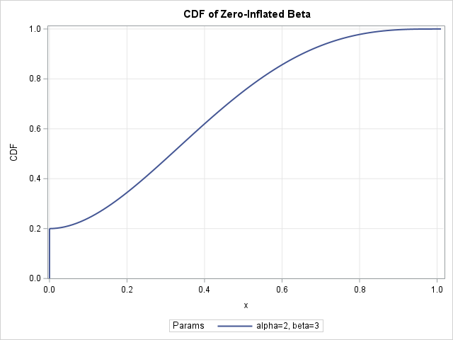
For any value of x along the horizontal axis, the graph shows the probability (on the vertical axis) that a random observation is less than or equal to x. For example, the function at x=0.4 shows that there is approximately a 63% chance that a random variate from that distribution will have a value less than or equal to 0.4. Notice that there is a 20% probability that a random observation is 0.
The ZI Beta quantile function
The quantile function is the inverse of the CDF function. Given a probability, p in (0,1), the quantile function at p is the x value such that a random observation drawn from the ZI Beta distribution will be less than or equal to x with probability p. For a ZI distribution, you can use the quantile function of the continuous distribution, but you need to rescale the probability to account for the point-mass at 0. The following DATA step calls the quantile_ZIBeta function, then uses PROC SGPLOT to visualize the quantile curves.
data Quantile_Test; %DefineParms; dp = 0.01; do p = 0 to 1-dp by dp, 0.999, 0.9999, 1; x = quantile_ZIBeta(p, p0, alpha, beta); output; end; keep p0 p x Params; run; title "Quantile Function of Zero-Inflated Beta"; proc sgplot data=Quantile_Test; series x=p y=x / group=Params lineattrs=(thickness=2); yaxis grid min=0 offsetmin=0; xaxis grid; run; |

Notice that the graph of the quantile function is the "flipped image" of the CDF graph. Notice also that the derivative of the quantile becomes infinite as x → 1. This is because the slope of the CDF function approaches 0 as x → 1.
Random variates from the ZI Beta distribution
For any mixture distribution, generating random variates requires two steps. The first step is to generate a binary random variate. (In SAS, this is done by using the "Bernoulli" distribution.) With probability π, you return a random variate from the first distribution; with probability 1-π, you return a random variate from the second distribution. For the ZI Beta distribution, this means that you return 0 with probability π, and a random variate from the Beta distribution with probability 1-π. If you draw a histogram of the resulting random variates, the bin that includes 0 will display the counts of the random variates near 0 from both distributions.
The following DATA step calls the rand_ZIBeta function 1000 times. Approximately 20% of the random variates are from the point-mass at 0. The remaining variates are from the Beta distribution.
data Rand_Test; %DefineParms; call streaminit(1234); N = 1000; do j = 1 to N; x = rand_ZIBeta(p0, alpha, beta); output; end; keep x Params; run; title "Random Variates for the Zero-Inflated Beta"; proc sgplot data=Rand_Test; histogram x; yaxis grid; xaxis grid; run; |

Because the program generates 1,000 random variates, the shape of the histogram is similar to the shape of the PDF curve. Specifically, note that bar that includes x=0 is slightly more than 20% for this random sample.
Define the functions for the ZI Beta distribution in SAS IML
Some programmers prefer to use the SAS IML language, especially when conducting a simulation study. Appendix 2 presents SAS IML module definitions. You can store the definition, then call them from a SAS IML program.
Summary
This article demonstrates how to implement a zero-inflated distribution in SAS. This article implements the zero-inflated Beta distribution, but you can use the same techniques for other zero-inflated distributions. Appendix A of this article defines four related functions in PROC FCMP in Base SAS: the PDF, CDF, quantile, and random variate functions. SAS IML versions of the functions are defined in Appendix B.
Appendix A: FCMP functions for the zero-inflated Beta distribution
This appendix shows how to use PROC FCMP in SAS to add new DATA step functions. It follows the same technique as a previous article about the generalized extreme-value (GEV) distribution. Run this PROC FCMP step before trying to call the functions in the DATA step.
/* Define the PDF, CDF, QUANTILE, and RAND functions for the ZI Beta distribution in PROC FCMP. The support for the ZI Beta distribution is X in [0,1). alpha : Shape1 > 0 beta : Shape2 > 0 For simplicity, the function assume alpha > 0 and beta > 0. The PDF is undefined if x=1 and beta < 1. It is well-defined for other parameter values. For simplicity, we always return a missing value with x=1. Thus, the variates for the distribution are defined on [0,1). */ proc fcmp outlib=work.funcs.ProbDist; function PDF_ZIBeta(x, p0, alpha, beta); if x < 0 | x >= 1 then return (.); f = ifn(x=0, p0, (1-p0)*pdf('Beta', x, alpha, beta)); return (f); endsub; function CDF_ZIBeta(x, p0, alpha, beta); if x < 0 | x >= 1 then return (.); F = ifn(x=0, p0, p0+(1-p0)*cdf('Beta', x, alpha, beta)); return (F); endsub; function quantile_ZIBeta(p, p0, alpha, beta); if p < 0 | p > 1 then return (.); if p <= p0 then return (0); if p = 1 then return (1); z = (p-p0)/(1-p0); /* rescale the probability on [p0,1] */ x = quantile('Beta', z, alpha, beta); return (x); endsub; function rand_ZIBeta(p0, alpha, beta); b = rand("Bernoulli", 1-p0); if b=0 then return (0); x = rand('Beta', alpha, beta); return (x); endsub; quit; options cmplib=work.funcs; /* define location of functions so the DATA step can find them */ |
Appendix B: SAS IML functions for the zero-inflated Beta distribution
This appendix shows how to define the PDF, CDF, QUANTILE, and RAND functions for the ZI Beta distribution in the SAS IML language.
proc iml; /* PDF of Zero Inflated Beta Distribution x can be a vector; p0, alpha, and beta are scalars. */ start PDF_ZIBeta(x, p0, alpha, beta); f = j(nrow(x), ncol(x), .); idx = loc(x = 0); if ncol(idx)>0 then f[idx] = p0; idx = loc(0 < x & x < 1); if ncol(idx)>0 then f[idx] = (1-p0)*PDF('beta', x[idx], alpha, beta); return f; finish; /* CDF of Zero Inflated Beta Distribution x can be a vector; p0, alpha, and beta are scalars. */ start CDF_ZIBeta(x, p0, alpha, beta); F = j(nrow(x), ncol(x), .); idx = loc(x = 0); if ncol(idx)>0 then F[idx] = p0; idx = loc(x = 1); if ncol(idx)>0 then F[idx] = 1; idx = loc(0 < x & x < 1); if ncol(idx)>0 then F[idx] = p0 + (1-p0)*CDF('beta', x[idx], alpha, beta); return F; finish; /* Quantile function of Zero Inflated Beta Distribution p can be a vector in (0,1); p0, alpha, and beta are scalars. */ start Quantile_ZIBeta(p, p0, alpha, beta); x = j(nrow(p), ncol(p), .); idx = loc(0 <= p & p <= p0); if ncol(idx)>0 then x[idx] = 0; idx = loc(p = 1); if ncol(idx)>0 then x[idx] = 1; idx = loc(p0 < p & p < 1); if ncol(idx)>0 then do; z = (p[idx]-p0)/(1-p0); /* rescale the probability on [p0,1] */ x[idx] = quantile('Beta', z, alpha, beta); end; return x; finish; /* Random variate function of Zero Inflated Beta Distribution N is the number or random variates; p0, alpha, and beta are scalars. */ start Rand_ZIBeta(N, p0, alpha, beta); x = j(N, 1, .); b = randfun(N, 'Bernoulli', 1-p0); idx = loc(b = 0); if ncol(idx)>0 then x[idx] = 0; idx = loc(b = 1); nBeta = ncol(idx); if nBeta>0 then x[idx] = randfun(nBeta, 'Beta', alpha, beta); return (x); finish; store module=(PDF_ZIBeta CDF_ZIBeta quantile_ZIBeta Rand_ZIBeta); QUIT; /* Test the functions for the ZI Beta distribution */ proc iml; load module=(PDF_ZIBeta CDF_ZIBeta quantile_ZIBeta Rand_ZIBeta); p0 = 0.2; alpha = 2; beta = 3; dx = 0.01; x = 0 // 1E-6 // T(do(dx, 1, dx)); PDF = PDF_ZIBeta(x, p0, alpha, beta); title "PDF of Zero-Inflated Beta"; call series(x, PDF) grid={x y}; title "CDF of Zero-Inflated Beta"; CDF = CDF_ZIBeta(x, p0, alpha, beta); call series(x, CDF) grid={x y} other="refline 0.2/axis=y; yaxis grid values=(0 to 1 by 0.1);"; title "Quantile Function of Zero-Inflated Beta"; dp = 0.01; p = T(do(0, p0, dp)) // T(do(p0+dp/10, 1, dp)); q = quantile_ZIBeta(p, p0, alpha, beta); call series(p, q) grid={x y}; title "Random Variates for the Zero-Inflated Beta"; x = Rand_ZIBeta(1000, p0, alpha, beta); call histogram(x) grid={y}; QUIT; |