One of the great algorithms of linear algebra is the Gram-Schmidt orthogonalization process, which enables you to construct an orthogonal basis for a linear subspace from any set of linearly independent vectors that span the subspace. The Gram-Schmidt process is the basis for the QR decomposition in numerical linear algebra, which decomposes any matrix, A, into a product, A = QR, where Q is a matrix with orthonormal columns, and R is an upper triangular matrix. In statistics, the QR algorithm can be used for linear least-squares regression, among other uses.
The ideas behind the orthogonalization process are simple: Project a vector onto a linear subspace and compute the residual vector. The residual vector is orthogonal to the subspace. Thus, these two operations decompose any vector into two parts: A vector that lies in the subspace and a vector that is orthogonal to the subspace. This article shows two subroutines in the SAS IML language that are useful for projecting a vector into a subspace and finding an orthogonal vector to a subspace. The GSORTH subroutine implements the Gram-Schmidt orthogonalization of a matrix, whereas the ORTVEC subroutine performs one step of the process and is useful for finding a orthogonal vector to a subspace.
The Gram-Schmidt orthogonalization of a matrix
Suppose V1, V2, ..., Vk are k linearly independent vectors. Let S = span(V1, V2, ..., Vk) be the linear subspace that they span. The Gram-Schmidt process uses these vectors to construct a set of orthogonal vectors for S. In SAS IML, you can put the vectors into the columns of a matrix and call the GSORTH subroutine. The subroutine takes one input argument (a matrix, V) and returns three output matrices. The output are as follows:
- Q: An orthonormal matrix whose columns contain an orthonormal basis for the subspace, S .
- T: An upper triangular matrix that transforms the orthonormal basis into the original basis: V = Q*T.
- lindep: A binary scalar value. If lindep=1, the columns of V are linearly dependent. If lindep=0, the columns of V are linearly independent, which implies dim(S) = k.
Here's an example. The columns of V span a 3-D linear subspace in the R4 Euclidean space.
proc iml; /* the columns of V span a 3-D subspace in R^4 */ V = { 1 1 0, -1 0 2, -1 1 -1, 1 1 2 }; call gsorth(Q, T, lindep, V); /* output: Q, T, and lindep from the input matrix, V */ print Q[F=BestD6.], T[F=BestD6.]; /* verify that V = Q*T by computing the difference V - Q*T */ maxDiff = max(abs(V - Q*T)); print maxDiff; |
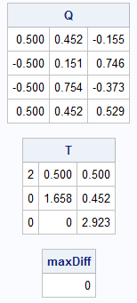
The original three basis vectors are V1={1, -1, -1, 1}, V2={1, 0, 1, 1}, and V3={0, 2, -1, 2}. They span a subspace, S, in R4. After calling the GSORTH routine, the columns of the matrix Q contain an orthogonal set of basis vectors that also span S. (To standardize the output, the columns of Q have unit norm, which means they form an orthonormal basis.) The T matrix maps one set of basis vectors onto the other. Specifically, V = Q*T is the equation that represents each column of V as a linear combination of the columns of Q. For this example, the columns of V are linearly independent, so lindep=0 and dim(S) = 3.
Notice that this Q matrix is not square, so it cannot be called an orthogonal matrix. Instead, a rectangular matrix with orthonormal columns is called a semi-orthogonal matrix. If, in addition, the columns have unit length, it is called a semi-orthonormal matrix.
Computing orthogonal vectors to a linear subspace: The manual way
The GSORTH subroutine enables you to compute an orthonormal basis with a single call. In linear algebra texts, the Q matrix is usually constructed sequentially. At each step, you create a new orthonormal basis vector from one of the original spanning vectors. To understand how the GSORTH and ORTVEC subroutines work, it helps to look at the manual calculations. In my linear algebra class, the Gram-Schmidt orthogonalization process was used so often that it is indelibly etched into my brain from performing endless calculations by hand! This section shows the tedious manual computations. The subsequent section uses the ORTVEC subroutine to simplify these computations.
The Gram-Schmidt process builds an orthogonal basis incrementally. Let's look at the SAS IML code. The original vectors are V1, V2, and V3, which are columns of a matrix, V. We use them to construct a new set of orthogonal vectors (U1, U2, and U3), which are columns of a semi-orthogonal matrix.
The process works step-by-step, projecting vectors onto the existing subspace and calculating the residual:
-
Step 1: The first orthogonal vector, U1, is simply the first original vector.
U1 = V1
 If you want to, you can standardize U1 construct an orthonormal basis, but let's keep it simple for now.
We'll standardize the U vectors at the end.
If you want to, you can standardize U1 construct an orthonormal basis, but let's keep it simple for now.
We'll standardize the U vectors at the end.
-
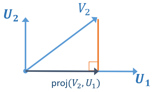
Step 2: The second orthogonal vector, U2, is the second original vector minus its projection onto the first orthogonal vector. Geometrically, you decompose V2 into two components, one lying in the span of U1 and the other orthogonal to it.
The orthogonal component becomes U2:
U2 = V2 - proj(V2, U1) -
Step 3: The third orthogonal vector is the third original vector minus its projections onto the first two orthogonal vectors.
Geometrically, you decompose V3 into two components, one lying in span(U1, U2) and the other orthogonal to it.
The orthogonal component becomes U3:
U3 = V3 - proj(V3, U1) - proj(V3, U2)
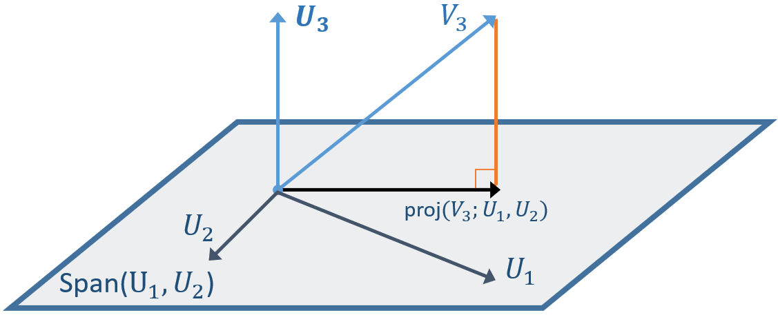
In these equations, the projection operator proj(y, x) calculates the projection of a vector y onto the line spanned by vector x.
Let's implement these three steps of the G-S orthogonalization process in the SAS IML language.
To make sure we get the same answer as the GSORTH subroutine, we can standardize the columns of U to form Q:
/* manual operation: project y onto span(x) */ start proj_vec(y, x); z = x/ norm(x); /* unit vector in direction of x */ return( (y`*z) * z ); finish; U = j(nrow(V), ncol(V), .); U[,1] = V[,1]; U[,2] = V[,2] - proj_vec(V[,2], U[,1]); U[,3] = V[,3] - proj_vec(V[,3], U[,1]) - proj_vec(V[,3], U[,2]); print U; /* optionally normalize the columns of U at each step or at the end. */ norm_vec = j(1, ncol(U), .); Q = j(nrow(U), ncol(U), .); do j = 1 to ncol(U); norm_vec[j] = norm(U[,j]); Q[,j] = U[,j] / norm_vec[j]; end; print norm_vec[F=Best5.], Q[F=BestD6.]; |
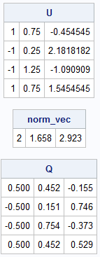
Notice that the Q matrix from these steps is identical to the Q matrix that is produced by the GSORTH subroutine. The U matrix is an "un-standardized" version of Q.
Computing orthogonal vectors to a linear subspace: The easier way
As described in the previous section, the Gram-Schmidt process is a series of operations that projects vectors onto a linear subspace, computes a vector orthogonal to the subspace, and then iterates. The ORTVEC subroutine encapsulates one step in this iterative process. It standardizes the orthogonal vectors at each step, thus forming the Q matrix directly instead of first forming U and then standardizing the columns.
The syntax for the ORTVEC routine is a little complicated. Let n be the dimension of the vectors (in our example, n=4). The input arguments for the ORTVEC subroutine are an n x 1 vector, v, and a semi-orthonormal n x k matrix, Q, where k ≤ n. This syntax is used for finding the (k+1)th orthonormal basis vector, based on the previous k orthonormal vectors. The vector v is the (k+1)th vector in the original basis. The ORTVEC routine returns four values: two vectors, w and r, a scalar rho, and a binary flag that tells you whether v is in the span of the columns of Q. The return values provide the decomposition of v into a component inside span(Q) and a component orthogonal to span(Q). In symbols, v = Q*r + rho*w, where norm(w)=1. The vector w is orthogonal to the span of the columns of Q. The vector w is the most important output from the ORTVEC subroutine.
To get the first orthonormal basis vector, you omit the Q matrix. This is shown in the following example, which uses the ORTVEC subroutine to compute the same Q vector as in the previous section:
/* the ORTVEC function in SAS IML performs several linear algebra operations related to G-S orthogonalization */ Q= j(nrow(V), ncol(V), .); call ortvec(w1,r,rho1,lindep, V[,1]); /* Step 1: No Q matrix yet; rho = norm(v1); v1 = rho1*w1 */ Q[,1] = w1; /* Check: v1 = rho1*w1; print (v1-V[,1]); */ call ortvec(w2,r2,rho2,lindep, V[,2], Q[,1]); /* Step 2: v2 = Q1*r2 + rho2*w2 */ Q[,2] = w2; /* Check: v2 = Q[,1]*r2 + rho2*w2; print (v2-V[,2]); */ call ortvec(w3,r3,rho3,lindep, V[,3], Q[,1:2]); /* Step 3: v3 = [Q1 Q2]*r3 + rho3*w3 */ Q[,3] = w3; /* Check: v3 = Q[,1:2]*r3 + rho3*w3; print (v3 - V[,3]); */ print Q; |
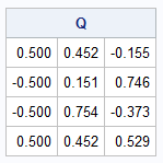
You now have three equivalent ways to construct the Q matrix. If you are interested in a programming challenge, you could put these ORTVEC operations into a DO loop (or a function) that performs the entire Gram-Schmidt orthogonalization algorithm for an arbitrary matrix, V. For an extra challenge, print out the sequence of 'r' vectors and the 'rho' scalars. Can you determine how they are related to the matrix T that is provided by the GSORTH routine?
Summary
The Gram-Schmidt orthogonalization algorithm enables you to construct an orthogonal basis for the span of other linearly independent vectors. The orthogonalization process decomposes every vector into a component that lies inside a subspace and a vector that is orthogonal to the subspace. In the SAS IML language, you can use the GSORTH subroutine to perform the full algorithm, or you can use the ORTVEC subroutine to perform one step. There are many applications that require finding a vector that is orthogonal to a subspace, so the ORTVEC subroutine is useful in these applications.