Estimate pi by tossing coins

Welcome to Pi Day 2026! Every year on March 14th (written 3/14 in the US), people in the mathematical sciences celebrate "all things pi-related" because 3.14 is the three-decimal approximation to π ≈ 3.14159265358979.... The purpose of this day is to have fun and celebrate the importance and ubiquity of pi.

This year's article shows a relationship between pi and simple game that involves a series of coin tosses. In a short, readable paper, Jim Propp (2026) describes a simple Monte Carlo method for estimating pi by tossing a coin. In this blog post, I use SAS to demonstrate the convergence by using a Monte Carlo simulation. I also explore the distribution of the statistic that estimates pi. But before you get all your friends together and start tossing coins, let me state clearly that this estimation method is not efficient in practice! This is an example of a mathematical result that is correct, but not efficient in practice.

The game: Toss a coin until there are more heads than tails

How can you flip a fair coin to estimate pi? Imagine a stadium filled with people. Each person has a fair coin and plays the following coin-tossing game:

Toss a coin and keep track of how many heads and tails appear.
Stop tossing as soon as the number of heads exceeds the number of tails.
Divide the total number of heads by the total number of tosses. Transmit this fraction to a moderator.

At the last step, each person sends their result to a moderator. (Nowadays, you would enter the numbers into a phone app!). The moderator (or app) computes the average of all the fractions of all the people in the stadium. The mathematical result by Propp is that the average of the fractions is π/4. Thus, if the moderator multiplies the average by 4, she obtains an approximation of pi.

Sequences and probabilities

Let's examine the coin-tossing process for each person in the stadium. First, notice that the total number of tosses is always odd. This is because the game stops as soon as the number of heads is one more than the number of tails. Here are some possibilities for the people in the auditorium:

About 1/2 (or 50%) of the people in the stadium toss the coin only once. They see heads on the very first coin toss. They are finished. They transmit the fraction 1/1 to the moderator.
1/8 (or 12.5%) of the people toss the coin three times. Their heads-and-tails sequence is THH. They transmit the fraction 2/3 to the moderator because they saw 2 heads after 3 tosses.
2/32 (or 6.25%) of the people toss the coin five times. Their sequence is either TTHHH or THTHH. They transmit the fraction 3/5 to the moderator.
5/128 (or 3.9%) of the people toss the coin seven times. They transmit the fraction 4/7 to the moderator. Their sequence is one of the following: TTTHHHH, TTHTHHH, TTHHTHH, THTTHHH, or THTHTHH.
In general, the fractions are all of the form (k+1) / (2k+1) for k=0, 1, 2, .... For a fair coin, Propp shows that the exact probability of the k_th fraction is $\binom{2k}{k} / (2 \cdot 4^k (k+1))$ . (In practice, a coin-flipper needs to transmit only the total number of tosses (t) because the number of heads is always (t+1)/2.)

The mathematical result: The expected value of a distribution

This section is very "mathy," so feel free to skip it and proceed to the next section where I show a SAS program that simulates the coin-tossing game to estimate pi.

Let X denote the random variable that represents the ratio "number-of-heads divided by number-of-tosses" for a random trial. (A "trial" is the complete sequence of tosses.) That is, values of X are the values x_k = (k+1) / (2k+1) with the above probabilities. Recall that the expected value of the discrete random variable is the sum E[X] = Σ x_k P(X=x_k). Propp noticed that the expected value for X is the Taylor series for (1/2)arcsine(1), which is π/4.

In other words,
$\pi/4 = 1/2 \cdot (1/1) + 1/8 \cdot (2/3) + 2/32 \cdot (3/5) + 5/128 \cdot (4/7) + ...$
and the probabilities 1/2, 1/8, 2/32, 5/128, ... can be estimated by using a large number of physical coin tosses or by using a computer simulation. This is a very cool result!

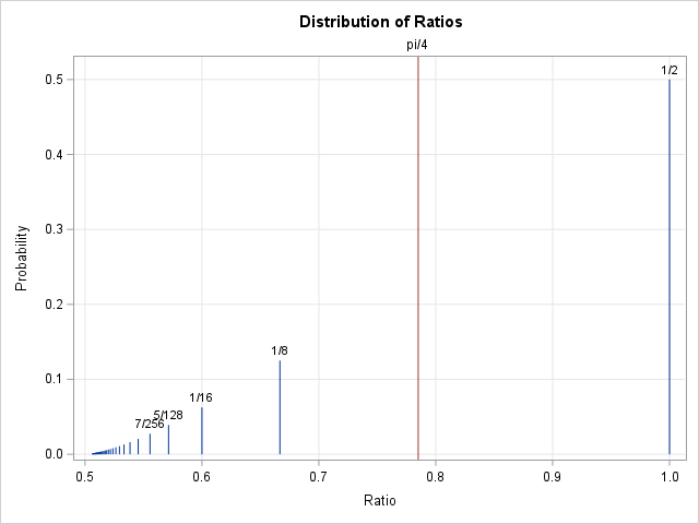
This is shown graphically in the plot to the right. (Click to enlarge.) Each vertical bar is located at a ratio that represents the number of heads divided by the number of coin tosses. The height of the bar is the probability that the ratio will occur in the coin-tossing game. The red vertical line is the quantity π/4. The mathematical result is that the π/4 is the weighted sum of all the ratios.

At this point a pure mathematician is satisfied. The series converges, the result is proved, end of discussion! But an applied mathematician is interested in the rate of convergence, and on that topic, there is bad news. As a general rule, Taylor series converge fastest near the center and slowest near the boundary of their disk of convergence. The Taylor series (about 0) for arcsine(x) converges for |x| ≤ 1, which means that the series is very slow to converge when x=1. Furthermore, because it is a series of positive terms, the partial sums approach π from below, and any finite summation is less than π.

How slow is the convergence? The following approximations give you some idea:

If you use four terms of the series (as written above), the estimate of π is 4*(0.62) = 2.483. This is not a very good approximation of pi!
If you use 10 terms of the series, the estimate is π ≈ 4*(0.691) = 2.764, which is still a bad approximation of pi.
If you use 100 terms of the series, the estimate is slightly more than 3: π ≈ 4*(0.757) = 3.028.
Even if you use 100,000 terms of the series, the estimate is only good to one decimal place: π ≈ 4*(0.7845) = 3.138.

In conclusion, this series is mathematically interesting but is not an efficient way to compute pi.

A Monte Carlo simulation to estimate pi

There are several Monte Carlo simulations that estimate pi, but now we have a new method: simulate many people tossing a coin until the number of heads is greater than the number of tails. You can write a simple DATA step in SAS to perform the Monte Carlo simulation, as follows:

/* Play the coin-tossing game to estimate pi (Propp, 2026) */
%macro CoinIsHeads;
   (rand("Bernoulli", 0.5)=1)
%mend;
 
%let numPeople = 1000;
data TossCoins;
call streaminit(123);
cusum = 0;
do trialID = 1 to &numPeople;          /* each person tosses a coin */
   nTails = 0;
   nHeads = 0;
   /* toss until the number of heads is greater than the number of tails */
   do while (nTails >= nHeads);        
      if %CoinIsHeads then nHeads + 1;
      else                 nTails + 1;
   end;
   n = nTails + nHeads;                /* total number of tosses */
   trial_ratio = nHeads / n;           /* the ratio nHeads/n for each trial */
   cusum + trial_ratio;                /* cumulative sum of ratios */
   pi_estimate = 4*cusum / trialID;    /* multiply by 4 so running mean = estimate of pi */
   output;
end;
run;
 
title "Running Average of Ratio nHeads/n";
%let pi = 3.14159265358979;
proc sgplot data=TossCoins;
   scatter x=trialID y=pi_estimate;
   refline &pi / axis=y label='pi' labelpos=min lineattrs=GraphData2;
   yaxis grid label="Estimate of pi";
   xaxis grid label="Number of Trials";
run;

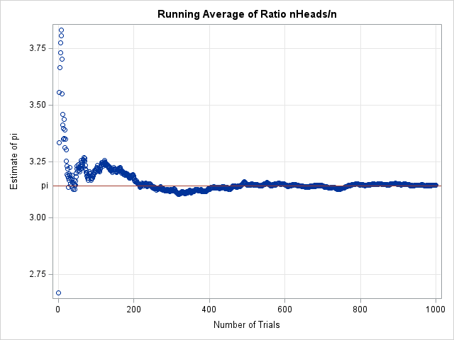
The graph shows the convergence of the estimate of π as you successively tabulate the results of 1,000 participants. For this random set of trials, the estimate starts large, but settles down after about 200 results. For the 1,000 participants in this trial, the final estimate is 3.14514, which is only two digits of accuracy. See Appendix 1 for a discussion of how the estimate might change if you repeat the experiment.

The number of trials is unbounded

There is a hidden inefficiency in this simulation. Notice that the innermost loop in the program is a DO-WHILE loop that simulates tossing a coin sequentially until the number of heads exceeds the number of tails. You might think that this inner loop runs a few dozen times, at most. But that's not true! A participant might get "unlucky" and start out by tossing a large number of tails, it might take hundreds or thousands of tosses before the number of heads exceeds the number of tails! You can use PROC UNIVARIATE to reveal the five largest number of trials in the simulation:

proc univariate data=TossCoins;
   var n;
   ods select ExtremeObs;
run;

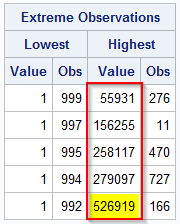
The column outlined in red shows the number of coin tosses for the most unlucky participants. These unfortunate coin-flippers tossed their coins many thousands of times until the number of heads exceeded the number of tails. The most unlucky participant tossed his coin 526,919 times! Clearly, this experiment not feasible in real life! See Appendix 2 to learn more about why you should expect arbitrarily large stopping times.

Summary

Propp (2026) proves an interesting mathematical result: You can use a series of coin flips to estimate π. The method involves a mathematical game where you toss a coin until the number of heads exceeds the number of tails. You can estimate π as the average of the ratio "number-of-heads divided by number-of-tosses." Asymptotically, as many people play this game, the estimate converges to π/4, which is the expected value of the distribution of the ratio. Just multiply the average by 4 to estimate π.

However, don't start flipping coins just yet! In practice, this process converges very slowly, and an unlucky coin-flipper might spend hours or days before the sequence of heads and tails shows more heads than tails.

Appendix 1: The variance of the estimate of pi

The main body of this article includes a graph of the running total of the estimate of pi when 1,000 people play the coin-tossing game. Of course, that is only one possible realization. If you ask these same 1,000 people to repeat the experiment, the result will be different because of random chance. The following graph shows 100 different instances of playing the same game.

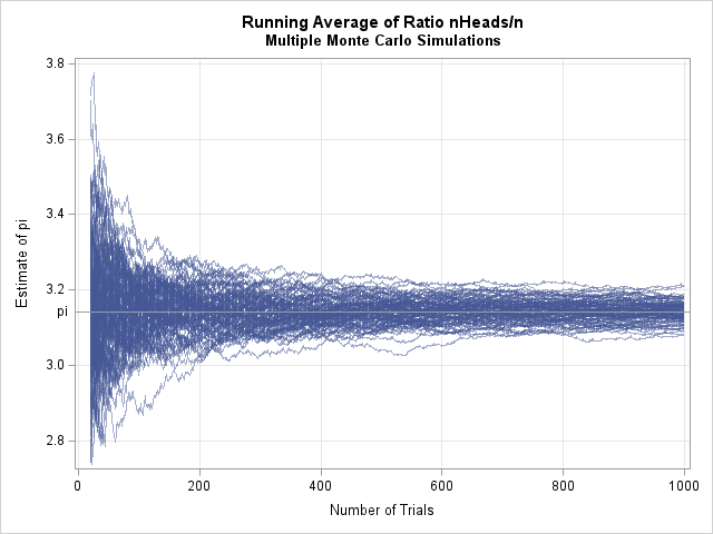
The values at the right side of the graph (n=1000) represent the estimates from each game. The average of those estimates is called the Monte Carlo estimate. For these trials, the Monte Carlo estimate of π is 3.1438, which is accurate to two decimal places. An empirical 95% confidence interval for that estimate is [3.090, 3.187].

Appendix 2: The stopping time of a discrete symmetric random walk

The coin-tossing game is a classic example of a one-dimensional symmetric random walk. In a symmetric random walk, we imagine an ant that starts at x=0 on a number line. With probability 1/2, the ant takes a random unit step to the left or right. What is the expected number of steps until the ant reaches x=1?

Random walks are well-studied. It is mathematically certain that the ant will eventually reach x=1, but you can prove that the expected stopping time is infinite. Returning to coin tosses, the game is guaranteed to end, but the number of coin flips before it ends is an unbounded quantity. If enough people play, some unlucky soul will pass out from exhaustion long before he reaches the stopping criterion.

Blogs