Stirling numbers in SAS

In probability and statistics, special numbers are used to compute probabilities by counting the number of ways certain events can occur. The most famous are combinations and permutations. Both are used to count the ways to arrange or select items from a set. If a set contains n elements:

A permutation is a sequence of the n elements. The order of the elements in the sequence is important. There are n! permutations of n distinct elements.
A combination of size k is a subset containing k elements. The number of combinations of size k, denoted by C(n,k) is equal to the binomial coefficient "n choose k". In a combination, the order of the elements is unimportant.

This article shows how to compute Stirling numbers of the second kind in SAS. (In this article "Stirling numbers" always means "of the second kind" because the "first kind" is less often encountered in probability.) Whereas combinations and permutations count arrangements of elements, Stirling numbers, denoted S(n,k), count the number of ways to partition a set of n elements into k non-empty and unlabeled subsets.

From the definition, a few special values for S(n,k) can be immediately identified:

S(n,n)=1 for n > 1. How many ways can you partition a set of n items into n (unlabeled) groups? There is only one way: Make n groups and put one element into each group.
S(n,1)=1. How many ways can you partition a set of n items into 1 group? There is only one way: Put all elements into the group.
S(n,0)=0 for n > 1. This is an edge case that is useful only for defining a recurrence relation between Stirling numbers. It's a silly question, but how many ways can you partition n items into 0 groups? That's not possible when n > 0, so we define S(n,0)=0 for n > 0. If n=0, we have a situation that involves empty sets. It is convenient to define S(0,0)=1, which means that there is one way to arrange zero items into zero sets.

A well-known example in probability theory is the coupon collector's problem, which calculates the probability of collecting a full set of n distinct coupons from random draws. You can use Stirling numbers in formulas for the probabilities.

SAS functions for combinatorics

In SAS, the FACT function returns the number of permutations for n distinct elements. The COMB function returns the number of combinations for choosing k out of n items. There are also built-in functions for computing the logarithm of these functions (LFACT and LCOMB, respectively). However, there is no built-in function for computing Stirling numbers.

Each of these combinatorial functions returns an integer value. In double precision numerical computations, integers values must fit into 8 bytes. Consequently, these functions return values less than constant("exactint") ≈ 9E15. This limits the size of the input to these functions. For examples, 18 is the largest input for the FACT function because 18! is less than 9E15 whereas 19! is not.

In this article, I provide two methods for computing Stirling numbers: An alternating summation formula and a formula that uses a recurrence relation. These formulas can be implemented in the DATA step, in a PROC FCMP function, or in a SAS IML function. For brevity, I show only the PROC IML functions.

The Stirling numbers as an alternating sum

According to the Wikipedia article on Stirling numbers, the definition involves an alternating sum that resembles a polynomial with terms that use the binomial coefficients:
$S(n,k) = \frac{1}{k!} \sum_{j=0}^{k} (-1)^{k-j} \binom{k}{j} j^{n} \quad \text{for } k \le n$

Because the formula involves a factorial, you should only use this formula for k less than or equal to 18. For larger values of k, you could calculate the ratio (sum/k!) by using logarithms as exp( log(sum) - log(k!) ), but you should round that expression to ensure it is an integer. The following SAS IML function implements the alternating-sum formula:

proc iml;
/* return S(n, k) the Stirling number of the second kind, which is the 
   number of ways to partition a set of n objects into k nonempty subsets.
   Note that 0 <= k <= n.
   S(n, k) = (1/k!) * sum_{j=0}^{k} (-1)^(k-j) * C(k, j) * j^n
   The input arguments are scalars; the output is also a scalar.
*/
start Stirling2(n, k);
   if n < k then return(0);  /* if n < k, S(n, k)=0  */
   if k = 0 then             /* if n > 0, S(n, 0)=0 */
      return choose(n=0, 1, 0);
 
   sum = 0;
   /* compute the summation. When n and k are large, 
      this alternating sum is not numerically stable */
   do j = 0 to k;
      sgn = choose( mod(k - j, 2), -1, 1);   /* +/- 1 */
      sum = sum + sgn # comb(k, j) # j##n;
   end;
   if k <= 18 then                           /* FACT(n) requires n<=18 */
      result = sum / fact(k);
   else
      result = exp(log(sum) - lfact(k));
   return( round(result) );                  /* output should be an integer */
finish;

The Wikipedia article includes a table that shows the Stirling numbers S(n,k) for all 0 ≤ k ≤ n ≤ 10. Let's call the IML function in a double loop to reproduce the table in SAS:

/* use alternating sum definition and a double loop to get all elements in matrix */
/* generate the "Table of Values" in Wikipedia:
   https://en.wikipedia.org/wiki/Stirling_numbers_of_the_second_kind#Table_of_values
*/
m = 10;
Stirling = j(m,m,0);
do n = 1 to m;
   do k = 1 to n;
      Stirling[n,k] = Stirling2(n, k);
   end;
end;
print Stirling[r=(1:m) c=(1:m)];

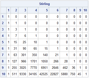
The output is identical to the table in Wikipedia.

From a computational perspective, there are two problems with the previous double loop:

To paraphrase Jerry Lee Lewis, "there's a whole lotta loopin' goin' on." In a matrix-vector language such as IML, it's more efficient to compute with vectors than to perform scalar computations in a loop.
The alternating-sum formula adds and subtracts big numbers. In numerical analysis, it is known that sums like this can lead to a severe loss of precision due to "catastrophic cancellation."

A recurrence relation for Stirling numbers

An alternative formula for Stirling numbers does not require computing an alternating sum. It is sometimes called "the recursive formula," but you can apply the formula iteratively. No recursion required! The formula results from the observation that Stirling numbers obey the following recurrence relation:
$S(n+1, k) = k S(n,k) + S(n,k-1) \quad \text{for } 0 \le k \le n$
and that the initial values for the formula are S(n,n)=1 and S(n,0)=0 for n > 1.

An advantage of the recurrence formula is that it can be vectorized. In the table of Stirling numbers, n indicates the row and k indicates the column. The formula tells us that the next row in the table can be constructed from the previous row. In the table, the k_th column of the next row is k times the value above it plus the value above and to the left of it. The diagram below shows how to apply the formula to compute the 5th row if you already know the 4th row:

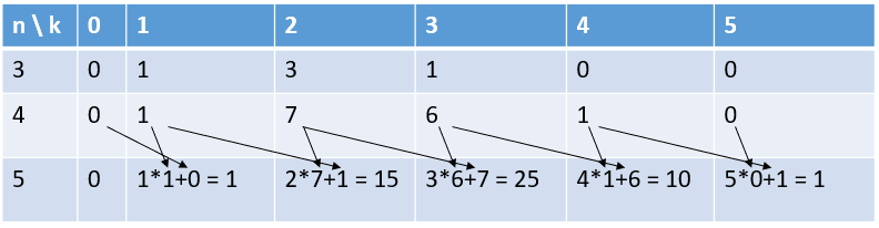
This method might remind you of the rows in Pascal's triangle, where the next row can be constructed by using the two values in the previous row.

The following SAS IML function implements the recurrence relation. If you want the n_th row of Stirling numbers, the function computes a total of n rows but returns only the last row that it computes:

/* You can use the recursion relationship to build the n_th row from the (n-1)th row:
   S(n,k) = k*S(n-1,k) + S(n-1,k-1) 
   This function returns an entire row at a time.
   Return the vector {S(n,1), S(n,2), ..., S(n,n)}
*/
start StirlingRow(n);
   Sn = 1;               /* first row: S1 = 1 */
   do q = 2 to n;
      k = 1:(q-1);
      /* pad with 0 to make rows the same size; overwrite S(n,.) with S(n+1,.) */
      Sn = (k#Sn || 0 ) +  ( 0 || Sn);   
   end;
   return Sn;
finish;
/* test the function by computing the rows for n=1 to 10 */
m = 10;
Stirling = j(m,m,0);
do n = 1 to m;
   Sn = StirlingRow(n);
   Stirling[n, 1:n] = Sn;    /* insert into larger matrix */
end;
print Stirling[c=(1:m) r=(1:m)];

The output is the same table as in the previous section. However, computing the elements row-by-row is vectorized. In addition, the algorithm avoids summing large terms that have different signs.

Of course, the previous implementation discards a lot of computations. If you ask for the 5th row, the function computes rows 1-4, but returns only the 5th row. If you plan to compute Stirling numbers for several values of n, it is more efficient to remember each row as you compute it and return a matrix of values, as follows:

/* If you want multiple rows (the entire matrix), you use the recursion relationship 
   and remember each row. This function returns an (n x n) matrix.
*/
start StirlingMat(n);
   Sn = 1;               /* first row: S1 = 1 */
   S = j(n,n,.);
   S[1,1] = Sn;
   do q = 2 to n;
      k = 1:(q-1);
      /* pad with 0 to make rows the same size; overwrite S(n,.) with S(n+1,.) */
      Sn = (k#Sn || 0 ) +  ( 0 || Sn);   
      S[q,1:ncol(Sn)] = Sn;
   end;
   return S;
finish;
/* test the function by computing the first 10 rows */
m = 10;
Stirling = StirlingMat(m);
print Stirling[c=(1:m) r=(1:m)];

The output is the same table as before, so it is not displayed,

Summary

This article shows how to compute Stirling numbers of the second kind in SAS. There is no built-in formula for these numbers, but you can implement a formula by using PROC IML (or PROC FCMP), The Stirling numbers count the number of ways that n items can be arranged into k subsets. These numbers can be used to compute probabilities for certain situations, such as the famous coupon collector's problem.

Blogs