The three-sigma rule

A remarkable result in probability theory is the "three-sigma rule," which is a generic name for theorems that bound the probability that a univariate random variable will appear near the center of its distribution. This article discusses the familiar three-sigma rule for the normal distribution, a less-familiar rule for unimodal distributions, and the most general rule that applies to all probability distributions (Chebyshev's inequality). The article includes simulation programs in SAS that demonstrate how to estimate the "k sigma" rule for any distribution and for any value of k.

The 68-95-99.7 rule for normal distributions

In an introductory class about probability, students often learn the "68–95–99.7 rule." This rule applies only to the normal distribution. It gives the probability that a normally distributed random variable is observed within 1, 2, and 3 standard deviations of the mean. The rule says that a random normal variate is observed within one standard deviation of its mean 68% of the time (or probability 0.68). A normal variate is observed within two standard deviations of its mean 95% of the time and within three standard deviations of its mean 99.7% of the time.

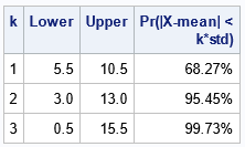
It is easy to use SAS to verify the 68–95–99.7 rule. If X ~ N(μ, σ) is normally distributed, then the probability that X is observed within k standard deviations of the mean is given by the integral of the density on the interval [μ - k σ, μ + k σ]. In terms of the cumulative distribution function, Φ, it is the difference Φ(μ + k σ) – Φ(μ - k σ). You can use the CDF function in SAS to verify the 68–95–99.7 rule for normal distributions:

/* validate the 68–95–99.7 rule analytically */
data ProbCoverageNormal(keep=k Lower Upper ProbCoverage);
mu = 8;         /* set the parameters for the normal distribution N(mu, sigma) */
sigma = 2.5;
mean = mu;      /* for the normal distribution, the mean is mu */
std  = sigma;   /* for the normal distribution, the std dev is sigma */
do k = 1 to 3;
   Lower = mean - k*std;
   Upper = mean + k*std;
   /* Pr(x \in [Lower, Upper]) */
   ProbCoverage = CDF("Normal", Upper, mu, sigma) -
                  CDF("Normal", Lower, mu, sigma);
   output;
end;
label ProbCoverage="Pr(|X-mean| < k*std)";
format ProbCoverage PERCENT8.2;
run;
 
title "Exact Coverage for the Normal distribution";
proc print data=ProbCoverageNormal label noobs;
run;

What is cool about the rule for normal distributions is that the coverage probability does not depend on the parameters μ or σ. Thus, for any parameter values, you could compute the probabilities by using the standard normal distribution: ProbCoverage = CDF("Normal", Upper) – CDF("Normal", Lower).

The value for k does not need to be an integer. It can be any positive number. Thus, you can ask for the probability that a normal variate is within 2.5 standard deviations of the mean (0.9876). Also, by subtracting the value from 1, you can obtain the probability that a variate is far from the mean. For example, the probability that a normal variate is farther than six standard deviations from the mean (the "six sigma rule") is 1.973E-09.

The three-sigma rule for other common distributions

Other distributions have similar "rules," although the coverage usually depends on the parameter values. For example, the coverage probabilities for the Gamma(2,2) distribution are 73.75%, 95.34%, and 98.59%. However, the probabilities for the Gamma(3,2) distribution are 75.10%, 93.64%, 98.26%. Notice that these values are different from the values for the normal distribution. It is a mistake to use the 68–95–99.7 rule if you do not have normally distributed data (see Wheeler, 2010).

In SAS, the CDF function supports dozens of common distributions. Therefore, if you know the theoretical distribution of the data, you can write a similar DATA step for any common distribution. To compute the coverage probabilities, you must write the mean and standard deviation in terms of the parameters. These formulas are often available on Wikipedia. For example, the mean and the standard deviation for the Gamma distribution can be written as:

mean = shape+scale;        /* mean of gamma(shape,scale) distrib */
std  = sqrt(shape)*scale;  /* SD of gamma(shape,scale) distrib */

Estimate the three-sigma rule in SAS

If you are interested in an obscure distribution that the CDF function in SAS does not support, you can use simulation to estimate the coverage probabilities. First, simulate a large random sample from the distribution. (I'll use N=10,000, but you get better estimates for N=100,000 or 1 million.) For each observation, count how many observations fall within one, two, and three standard deviations of the mean. Ideally, you would use the mean and standard deviation from the distribution, but you could use the sample mean and standard deviation if the population parameters are unknown. You then estimate the coverage probability as the proportion of variates that were observed in each interval.

The following SAS DATA step performs a simulation study for the normal distribution. In this case, we know the exact mean and standard deviation, so we use the parameters to construct the intervals [mean - k*SD, mean + k*SD]for k=1, 2, and 3. Notice a cool DATA step trick: I name TWO data sets on the DATA statement and use the "OUTPUT name" statement to write the simulated data to one data set and the estimated probabilities to the other:

%let N = 10000;    /* sample size */
data SimNormal(keep=y inSigma:)    /* NOTE: Two output data sets! */
     EstProbCoverNormal(keep=k Lower Upper EstProbCoverage);
mu = 8;
sigma = 2.5;
mean = mu;      /* for the normal distribution, the mean is mu */
std  = sigma;   /* for the normal distribution, the stddev is sigma */
call streaminit(12345);
array inSigma[3] (0 0 0);      /* count number of obs in each interval */
array aLower[3] _temporary_;   /* lower endpoint = mean - k*std for k=1,2,3 */
array aUpper[3] _temporary_;   /* upper endpoint = mean + k*std for k=1,2,3 */
do k = 1 to dim(aLower);
   aLower[k] = mean - k*std;   /* compute intervals for k=1,2,3 */
   aUpper[k] = mean + k*std;
end;
do i = 1 to &N;
   y = rand("Normal", mu, sigma);
   do k = 1 to dim(inSigma);
      /* count number of variates in [Lower, Upper] */
      inside = (aLower[k] < y < aUpper[k]);  /* 0 or 1 */
      inSigma[k] + inside;
   end;
   output SimNormal;           /* save the random variates to one data set */
end;
/* after simulating N variates, estimate probabilities by using proportions */
do k = 1 to dim(inSigma);
   Lower = aLower[k];
   Upper = aUpper[k];
   EstProbCoverage = inSigma[k] / &N;
   output EstProbCoverNormal; /* save the statistics to the other data set */
end;
run;

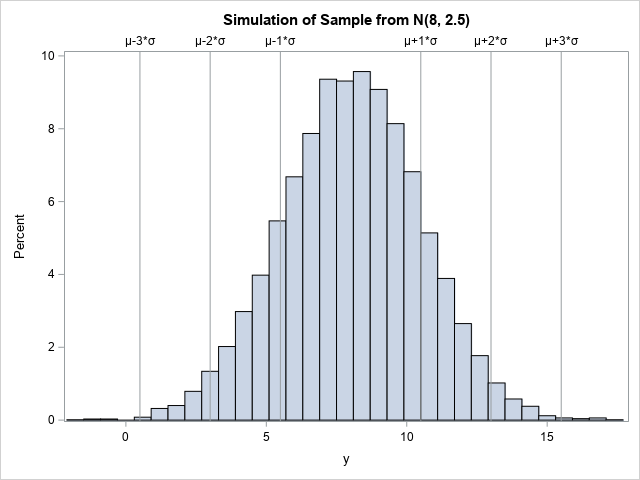
You can visualize the distribution of the sample in the SimNormal data set. The following statements call PROC SGPLOT to create a histogram and use the REFLINE statement to add a visual indication of the three intervals [μ-k*σ, μ+k*σ] for k=1,2, and 3.

/* visualize the data and coverage intervals */
%let mu    =(*ESC*){Unicode mu};
%let sigma =(*ESC*){Unicode sigma};
title "Simulation of Sample from N(8, 2.5)";
proc sgplot data=simNormal;
   histogram y;
   refline 5.5 10.5 3.0 13.0  0.5 15.5 / axis=x 
           label=("&mu-1*&sigma" "&mu+1*&sigma"
                  "&mu-2*&sigma" "&mu+2*&sigma"
                  "&mu-3*&sigma" "&mu+3*&sigma");
run;

The other data set (ProbCoverNormal) contains estimates for the coverage probabilities:

title "Monte Carlo Estimate Coverage for the Normal distribution";
proc print data=ProbCoverNormal label noobs;
   label EstProbCoverage="Est Pr(|X-mean| < k*std)";
   format EstProbCoverage PERCENT8.2;
run;

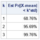
For this sample, the estimated probabilities agree with the exact probabilities to one decimal place. You can obtain more accuracy by using a larger sample size.

A three-sigma rule for unimodal distributions

Pukelsheim (TAS, 1994) wrote a nice article about theorems that describe the probability that a random observation is far from some location. As we have discussed, often the location is the mean of the distribution, but it doesn't have to be. For a unimodal distribution, you might be interested in the distance from the mode. Gauss proved a theorem that bounds the probability that a random variate is far from the mode (Gauss's inequality).

Vysochanskij and Petunin (1980), improved Gauss's bound for general unimodal distributions. If X is a random variable from a unimodal distribution whose mode is ν, then Vysochanskij and Petunin proved that Pr(|X-ν| <= k*σ) ≥ 1 - (4/9)/k**2. Thus, for a unimodal distribution:

At least 55.6% of observations are within one standard deviation of the mode.
At least 88.9% of observations are within two standard deviations of the mode.
At least 95.06% of observations are within three standard deviations of the mode.

Notice that these numbers are lower bounds. The normal distribution is unimodal, and the mode is located at the mean. The coverage probabilities of the normal distribution are larger than these numbers. Nevertheless, it is useful to know that for ANY unimodal distribution, at least 95% of the probability is within three standard deviations of the mode!

A three-sigma rule for any probability distribution

In my opinion, one of the most amazing theorems in probability theory is Chebyshev's inequality. Chebyshev's inequality (sometimes called Chebyshev's theorem) provides a lower bound for the probability that a univariate random variate is within k standard deviations from the mean. The probability is at least 1 – 1/k². Equivalently, there is at most a probability of 1/k² that an observation is more than k standard deviations from the mean.

This is an amazing result because it is true for every probability distribution. It doesn't depend on whether the distribution is symmetric, skewed, bounded, unbounded, discrete, or continuous. The only requirement is that the probability distribution has a finite mean and variance.

Thus, for any univariate probability distribution with finite variance:

At least 0% of observations are within one standard deviation of the mean. (Okay, so k=1 isn't very interesting!)
At least 75.0% of observations are within two standard deviations of the mean.
At least 88.9% of observations are within three standard deviations of the mean.
You can consider higher values of k. For example, the "six sigma rule" is that at least 97.2% of observations are within six standard deviations of the mean. Equivalently, no more than 2.78% are farther than six standard deviations.

Some statisticians decry the theorem as being useless in practice. As mentioned, most common distribution have probabilities that are higher than the Chebyshev bounds. Nevertheless, it is a beautiful theoretical result! It quantifies why the mean is often considered the "center" of a distribution, and why the standard deviation is a natural scale to compare distances to the mean. Chebyshev's inequality has several generalizations, including a generalization to multivariate distributions.

Summary

There are several theorems in probability that ensure that most observations are close to the mean or mode of a univariate distribution. Chebyshev's theorem is the most general; it applies to any distribution that has finite variance. Vysochanskij and Petunin (1980) proved a comparable result that applies to any unimodal distribution and bounds the probability that an observation is far from the mode. There are also specific calculations, such as the 68–95–99.7 rule for the normal distribution, that tell you the probabilities that an observation is close to (or far from) the mean, or any other location.

References

Pukelsheim, F. (1994), "The Three Sigma Rule", The American Statistician.
Vysochanskij, D. F., and Petunin, Y. I. (1980), "Justification of the 3-sigma rule for Rule for Unimodal Distributions," Theory of Probability and Mathematical Statistics.
Wheeler, D. J. (2010). “Are You Sure We Don’t Need Normally Distributed Data? More about the Misuses of Probability Theory.” Quality Digest Daily.

Blogs