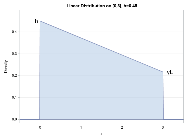
In a recent Monte Carlo project, I needed to simulate numbers on an interval by using a continuous linear probability density function (PDF). An example is shown to the right. In this example, the linear density function is decreasing on the interval, but the function could also be constant or increasing. This article derives the formulas for PDF, the cumulative distribution function (CDF), and the quantile function (inverse CDF) for a linear distribution. It shows how to generate random samples from the distribution by using the inverse CDF method for simulating from a distribution.
The linear distribution
I am sure that this bounded distribution has been studied before, but I couldn't find an online treatment. Perhaps it is included as an example or exercise in a probability textbook. The linear distribution in this article allows the density at one or both endpoints to be positive. This makes the linear distribution different from the triangular distribution and the trapezoidal distribution, since both of those distributions assume that the density function is 0 at both ends of the interval.
To the casual observer, the linear distribution has four parameters: the endpoints of the interval [a,b] and the values of the density function at each endpoint. However, like every probability distribution, the density must integrate to 1 on [a,b]. In addition, without loss of generality, you can set the left endpoint of the interval to 0 and consider only the length of the interval as a parameter. Thus, you can parameterize the distribution by using the length of the interval, L, and the height of the density function, h, at the left hand side of the interval. To be a proper probability distribution that is linear on [0,L], h must be in the interval 0 ≤ h ≤ 2/L.
If you specify L and 0 ≤ h ≤ 2/L, the rest of the distribution is determined, including whether the slope of the PDF is positive, negative, or zero. In the general case, the area under the PDF is a trapezoid, so the area is A = (h + yL)*L/2, where yL is the height of the density at the right hand side of the interval. This area equals 1, so yL = 2/L - h. Note that yL ≥ 0 because h ≤ 2/L.
Putting these facts together, you can write down the formula the PDF on [0,L] as
f(x; L, h) = m*x + h
where m = (yL - h) / L and yL = 2/L - h.
Implement the linear distribution PDF in SAS
You can implement the linear distribution in SAS by using the DATA step, the SAS IML Language, or PROC FCMP. The following statements define a SAS IML module that evaluates the PDF for x in the interval [0,L]. The function has only minimal error checking. For example, a more robust module would return 0 if x is not in [0,L].
/* Define a linear distribution on the interval (0,L). The height of the PDF at x=0 is h, where 0 <= h <= 2/L. This determines the height at x=L, which is yL = 2/L - h, which is nonnegative. Check the area to verify that the function defines a distribution on [0,L]. The trapezoidal area under the line is A = (h + yL)/2 * L = (h + (2/L - h))/2 * L = 1 as required */ proc iml; /* PDF of linear distribution on [0,L], where PDF(x=0) = h and 0 <= h <= 2/L ASSUME x in [0,L] (otherwise, need additional IF-THEN logic) */ start PDFLinear(x, L, h); if h > 2/L then return(.); /* invalid */ yL = 2/L - h; m = (yL - h) / L; pdf = m*x + h; return pdf; finish; L = 3; /* constrains h to 0 <= h <= 2/3 */ %let h = 0.45; h = &h; x = do(0, L, L/100); PDF = PDFLinear(x, L, h); title "Linear Distribution on [0,3], h=&h"; call series(x,PDF) grid={x y} other="yaxis grid min=0"; |
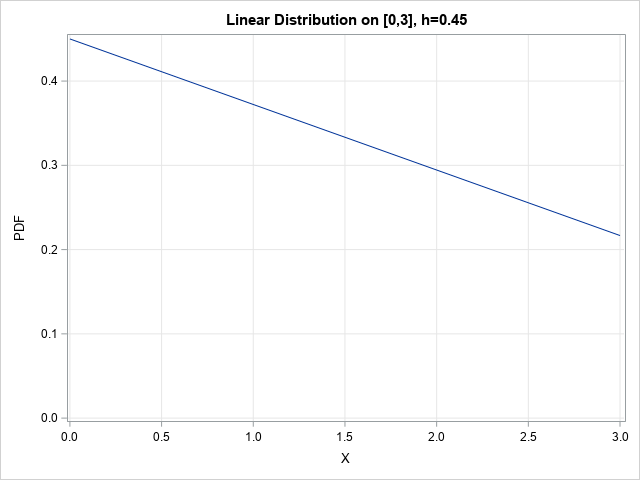
The graph of the density function agrees with the visualization at the top of this article.
Implement the linear distribution in SAS
From the PDF you can obtain the CDF, quantile function (inverse CDF), and random sampling:
- Obtain the CDF by integration. Since the PDF is linear, the CDF is an increasing quadratic function on [0,L].
- You can obtain the quantile function by finding the value of x for which u = CDF(x), where u is in [0,1]. Because the CDF is quadratic, you can use the quadratic formula to invert the CDF.
- To obtain a random variate, use inverse CDF sampling. Generate a uniform random variate u ~ U(0,1), then evaluate the quantile at u.
The following statements define functions for the CDF, quantiles, and random variates:
/* CDF of linear distribution on [0,L]. ASSUME x in [0,L] (otherwise, need additional IF-THEN logic) */ start CDFLinear(x, L, h); if h > 2/L then return(.); /* invalid */ yL = 2/L - h; m = (yL - h) / L; cdf = m*x##2 / 2 + h*x; return cdf; finish; /* Quantile function (inverse CDF) of linear distribution on [0,L] */ start QuantileLinear(u, L, h); if h > 2/L then return(.); /* invalid */ yL = 2/L - h; m = (yL - h) / L; if abs(m) < 1E-16 then /* m=0 so function is constant */ return u / h; discrim = h**2 + 2*m*u; return (-h + sqrt(discrim)) / m; finish; /* Random sample of linear distribution on (a,b) Uses inverse CDF method: generate u ~ U(0,1) and call quantile function. */ start RandLinear(n, L, h); u = randfun(n, "Uniform"); return QuantileLinear(u, L, h); finish; /* generate a random sample */ call randseed(1234, 1); n = 1000; x = RandLinear(n, L, h); title "Random Sample from Linear Distribution (h=&h)"; call histogram(x); |
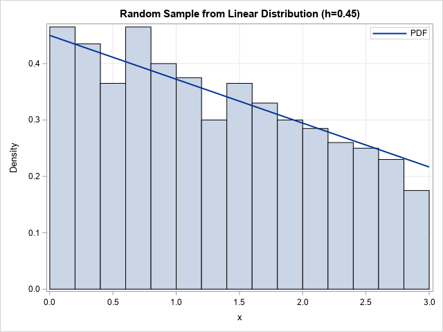
The SAS IML program displays only the histogram of the random sample of size 1,000. However, with additional effort you can overlay the PDF on the histogram, as shown in the preceding graph.
Increasing, decreasing, and constant distributions
The previous example shows a decreasing density function. Whether the density function is increasing, decreasing, or constant depends on the value of h relative to L.
- If h < 1/L, then the density function is increasing.
- If h = 1/L, then the density function is constant.
- If h > 1/L, then the density function is decreasing.
In the SAS program, I used a macro variable to define h. Because L=3, the critical value for h is h=1/3. You can set the macro variable to be 0.25, 0.333, and 0.45 to see examples of an increasing density, a constant density, and a decreasing density.
For the extreme cases where h=0 or h=2/L, the linear distribution simplifies to an increasing or decreasing triangular distribution, respectively.
Summary
I was unable to find an online description of a linear distribution on a closed interval, so I derived it in this article. The linear distribution is similar to the triangular distribution and the trapezoidal distribution, but it enables you to specify a nonzero density at the endpoints of the interval.
There are several useful ways to parameterize the distribution. I used the parameters L (the length of the interval) and h (the height of the PDF at the left-hand endpoint). It is also possible to define the distribution by using the height of the right-hand endpoint as a parameter. I leave that derivation as an exercise.
In this article, the support of the distribution is [0, L]. There is no loss of generality in using 0 for the left endpoint because if f(x) is the PDF for x in [0, L], then f(x-c) is the linear distribution on the interval [c, c+L]. Similarly, you can get random variates on [c, c+L] by generating random variates on [0, L] and adding c to each variate.
