The collinearity problem is to determine whether three points in the plane lie along a straight line. You can solve this problem by using middle-school algebra. An algebraic solution requires three steps. First, name the points: p, q, and r. Second, find the parametric equation for the line that passes through q and r. Third, plug in the coordinates of the third point, p. If the left and right sides of the equation are equal, then p lies on the line. If the p does not lie on the line through q and r, you can even figure out if p is above or below the line.
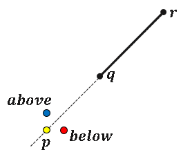
The geometry of the collinearity problem is shown in the figure to the right. The point p could be anywhere, but three possible locations are depicted. The yellow point is on the line through q and r. The blue point is above the line; the red point is below the line. We want to classify any point, p, as being on, above, or below the line.
Although the math is elementary, the numerical solution of this problem is surprisingly complex. Due to finite precision arithmetic, the left and right sides of the linear equation might not be equal when you plug in p, even if they the points are collinear in exact arithmetic. Even worse, you can choose coordinates for p that are not on the line through q and r, but the finite-precision computations mistakenly conclude that the points are collinear.
This article shows a simple example of testing three points for collinearity. As you slightly change the coordinates of the test point, the algorithm gives the wrong answer in surprising ways. The example is one of several interesting examples discussed in Kettner, Mehlhorn, Pion, Schirra, Yap (2008), "Classroom examples of robustness problems in geometric computations," Computational Geometry. The example I present is from p. 4-5.
An elementary computation for collinearity
Let's formulate a test to determine whether three planar points are collinear. There are many ways to do this, but I like to
find the area by using the determinant of a 3 x 3 matrix. To understand how a matrix appears, embed the planar points in 3-D space in the plane {(x,y,z) | z=1}. Now consider the points as 3-D vectors. The vectors form a tetrahedron when they are in general position. If the volume of the tetrahedron is 0, then the vectors are linearly dependent and the original three points are colinear. In terms of linear algebra, the volume is found as the determinant of the 3 x 3 matrix
\(V = \det \begin{pmatrix} p_1 & p_2 & 1 \\ q_1 & q_2 & 1 \\ r_1 & r_2 & 1 \end{pmatrix}\),
where (p1, p2), (q1, q2), and (r1, r2)
are the coordinates of the three points.
If the determinant is 0, then p is on the line through q and r. Furthermore, you can use the sign of the determinant (positive or negative) to determine whether p is above or below the line. The following SAS IML function returns the values 0 if the three points are numerically collinear. Otherwise, it returns +1 or -1, which we can interpret as "above" or "below."
proc iml; /* Return: 0 if three points are collinear +1 if points bend to the left -1 if points bend to the right */ start Orientation(p,q,r); /* theoretically, the operation is sign( det(M) ) */ return sign( (q[1] − p[1])*(r[2] − p[2]) −(q[2] − p[2])*(r[1] − p[1]) ); finish; /* test the function: p, q, and r are on the diagonal line y=x */ p = {0.5 0.5}; q = {12 12}; r = {24 24}; orientLine = Orientation(p, q, r); orientLeft = Orientation(p+{0 0.5}, q, r); /* shift p up */ orientRt = Orientation(p+{0.5 0 }, q, r); /* shift p to the right */ print orientLine orientLeft orientRt; |

The program illustrates the three cases in the figure at the top of this article. When the three points are perfectly collinear, the function returns 0. When p is shifted to be above the line through q and r, the function returns +1. When p is shifted to be below the line, the function returns -1.
Small perturbations can change the decision
The computation is simple, but small changes in the position of p can lead to unexpected changes. For example, let p=(0.5, 0.5), q=(12, 12), and r = (24, 24). These points are on the identity line y=x. If you move the point p up by any amount, the function should return +1 (in exact arithmetic). The previous section shows that the function does return +1 when you shift p by 0.5, which is a relatively large quantity. But what happens if you shift up p by a very small amount? The following program shifts up p by 2*ε, 5*ε, 10*ε, and 25*ε, where ε is "machine epsilon," which is approximately 2.22E-16 on my computer:
eps = constant('maceps'); /* 2.22E-16 */ p1 = p + {0 2}*eps; /* shift up by 2 units */ p2 = p + {0 5}*eps; /* shift up by 5 units */ p3 = p + {0 10}*eps; /* shift up by 10 units */ p4 = p + {0 25}*eps; /* shift up by 25 units */ orient_02 = Orientation(p1, q, r); orient_05 = Orientation(p2, q, r); orient_10 = Orientation(p3, q, r); orient_25 = Orientation(p4, q, r); print orient_02 orient_05 orient_10 orient_25; |
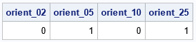
For a very small perturbation (2*ε), the function returns 0, which means that it decides that p is still on the line. But that's a very small perturbation, so perhaps we can forgive the computation for its error. For a larger perturbation (5*ε), the algorithm correctly concludes that the points are not collinear. \Great! So now you might expect all larger perturbations to result in the same conclusion. But they don't! When you shift up by 10*ε, the computation incorrectly claims that the points are collinear once again. When you shift by 25*ε or more, the computation correctly claims that the points are not collinear.
A similar situation occurs if you shift the point p to the left or right by adding small amounts to its first (x) coordinate.
Visualizing the collinearity results
To better understand the behavior of the collinearity computation, let's use a heat map to visualize the results for a systematic set of permutations of the point p. That is, let's vary the coordinates of p by adding perturbations of the form ε*(i,j), where (i,j) is a pair of integers. Let's look at the perturbations where -100 ≤ i,j ≤ 100. For each point of the form p + ε*(i,j), call the Orientation function and remember the result. Then plot the result as a discrete heat map. The heat maps has a cell for each (i,j) pair. The color of the cell shows whether the Orientation function returned 0, +1, or -1.
/* consider perturbations of the form p + eps*(i,j) for -100 <= i,j <= 100 */ eps = constant('maceps'); /* 2.22E-16 */ pert = expandgrid( -100:100, -100:100 ); orient = j(nrow(pert), 1, .); do k = 1 to nrow(pert); orient[k] = Orientation(p+pert[k,]*eps, q, r); end; /* write results to a SAS data set in long form */ i = pert[,1]; j = pert[,2]; create NumerOrient var {'i' 'j' 'Orient'}; append; close; QUIT; /* Create a discrete heat map: https://blogs.sas.com/content/iml/2019/07/15/create-discrete-heat-map-sgplot.html Reproduce the colors from Kettner, et al. (2008) */ proc format; value OrientFmt 0 = "Straight Line" 1 = "Left Bend" -1 = "Right Bend"; run; ods graphics / width=480px height=480px; title "Numeric Determination of Collinearity"; title2 "Perturbation by (eps*i, eps*j)"; proc sgplot data=NumerOrient aspect=1; format Orient OrientFmt.; styleattrs datacolors=(Yellow ModerateBlue ModerateRed); heatmapparm x=i y=j colorgroup=Orient / name="heat"; lineparm slope=1 x=0 y=0; keylegend "heat"; run; |
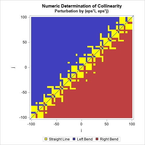
This image my version of Figure 2a of Kettner, et al. (2008, p. 5). You can observe several facts from the figure:
- In exact arithmetic, we would expect the cells to be blue in the upper-left triangular region, yellow on the (anti-)diagonal (collinearity), and red in the lower-right triangular region. In floating point arithmetic, the image is yellow for cells on the diagonal, but also yellow for some cells that are off the diagonal.
- You might expect the yellow cells to be clustered near the diagonal, but they aren't. For example, there is a set of yellow cells near (i,j)=(-25,10) which are completely surrounded by blue cells. Similarly, notice the cluster of cells near (i,j)=(-10,25). There are corresponding clusters of yellow in the red region.
- You might expect all the blue cells to be above the diagonal and all red cells to be below the diagonal, but they aren't. For example, there is a cluster of blue cells below the diagonal near (i,j)=(25,22). Nearby, you can spot some red cells above the diagonal.
One thing is clear: The numerical finite-precision computations to determine collinearity are not as simple as the exact-arithmetic computations.
How to handle issues like this
The heat map in the previous section demonstrates that even a simple computation is subject to finite-precision errors. The algorithm cannot robustly determine whether three points in the plane are collinear. This problem is not confined to this special example. Kettner, et al. (2008) show similar heat maps for several different choices of coordinates for the points p, q, and r. They also discuss other algorithms in computational geometry that have similar finite-precision issues.
The first step to solving a problem is acknowledging that there is a problem, which is the purpose of this article. It can be helpful to redesign your algorithms to avoid relying on the equality of floating-point values. Instead, test whether the three points are nearly collinear. For example, you could rewrite the Collinearity function to return 0 if the computation is in the range [-δ, δ] for a suitable small value of δ > 0. Equivalently, you can test whether the three points form a triangle that has a very small area. You should probably standardize the data so that, for example, the length of the longest side is 1.
An alternative algorithm is to test angles instead of area. For example, you could test whether every angle, θ, in the triangle satisfies |sin(θ)| < δ.
Summary
This article implements a function that tests three points for collinearity. The function is simple to implement and works flawlessly in exact arithmetic. However, the real world is not so simple. A perturbation analysis reveals that this simple function is subject to the complexities of finite-arithmetic computations. Kettner, et al. (2008) discuss this problem in greater detail. Acknowledging that there is a problem is the first step to solving it. For robust results, implement your algorithms to account for finite-precision calculations.
Appendix
The astute reader might wonder why I didn't use the built-in DET function in SAS IML to calculate the quantity sign(det(M)). The answer is that the DET function has built-in logic that makes robust decisions about whether a matrix is singular. Accordingly, if you use the DET function, the heat map shows a yellow strip of cells along the anti-diagonal with blue cells above and red cells below. Thus, the DET function will return 0 if the numerical determinant is in the range [-δ, δ] for a suitable small value of δ > 0. This is stated in the documentation for the DET function.
