Construct an envelope function for the acceptance-rejection method

The acceptance-rejection method (sometimes called rejection sampling) is a method that enables you to generate a random sample from an arbitrary distribution by using only the probability density function (PDF). This is in contrast to the inverse CDF method, which uses the cumulative distribution function (CDF) to generate a random sample. For many distributions, the CDF does not have a formula and can be computed only by numerically integrating the PDF, which is an extremely expensive computation. By using the acceptance-rejection method instead, you can avoid the numerical integration.

Of course, nothing is free. For the acceptance-rejection method, each time you generate a potential random variate, you need to perform a test to see whether the variate should be accepted or rejected. If the acceptance rate is low, it can take a long time to generate a random sample.

This article discusses how to use an acceptance-rejection method to generate a random sample from the Andrews distribution. After reviewing the efficiency of the simplest acceptance-rejection method, we improve the efficiency by constructing a nontrivial envelope function for the Andrews PDF. We show that well-chosen envelope function can greatly improve the efficiency of the acceptance-rejection method for simulating data from a distribution. The discussion includes a SAS program that illustrates the main ideas.

The simple acceptance-rejection method

Let's construct an example to demonstrate the acceptance-rejection method and to demonstrate why it can be inefficient. In a previous article, I constructed the PDF for a new distribution, which I called the Andrews distribution. The Andrews PDF is defined as f(x) = (1/S) sin(π x)/(π x) on the interval [-1, 1] and f(x) = 0 otherwise, where S=1.1789797. The CDF does not have a closed-form expression in terms of elementary functions, so let's use a simple acceptance-rejection algorithm to generate random samples. The simple algorithm is to generate a variate, x, uniformly at random on the interval [-1, 1], then accept x with probability f(x) / max(f), where max(f) = 1/S = 0.848 is the maximum value of the PDF, as shown by the following SAS DATA step implementation:

/* a simple acceptance-rejection algorithm that uses the horizontal line
   y = max(f) = 1/S = 0.848191 
   as an upper bound for generating random variates.
   The area of the bounding box is 2*(1/S), so the Pr(Accept) = S/2 = 0.5895.
*/
%let N = 10000;
data RandAndrews1;
S = 1.1789797;
call streaminit(1234);
pi = constant('pi');
maxf = 1 / S;                       /* max(f) */
numRand = 0;                        /* numRand = number of potential variates */
i = 0;                              /* i = number of accepted variates */
do while(i < &N);
   x = rand('Uniform', -1, 1);      /* potential variate x ~ U(-1,1) */
   numRand = numRand + 1;
   if x=0 then f = 1/S;             /* evaluate f(x) */
   else f = sin(pi*x) / (pi*x) / S;
   y = rand('Uniform', 0, maxf);    /* y ~ U(0,max(f)) */
   if y < f then do;                /* accept x with probability f(x) / max(f) */
      i = i + 1;                    /* x is accepted; increment counter */
      output;
   end;
end;
keep x i numRand;
call symputx('AcceptFrac', round(&N / numRand, 0.0001));
run;
 
title "Random Sample from Andrews Distribution";
title2 "Acceptance Rate = &AcceptFrac";
proc sgplot data=RandAndrews1;
   histogram x / scale=Percent;
   yaxis grid;
run;

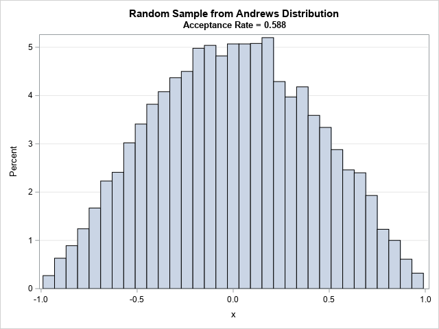
The output shows 10,000 random draws from the Andrews distribution.

The geometry of the simple acceptance-rejection method

How does the simple acceptance-rejection method work? The previous DATA step computes the proportion of uniform variates that are retained in a random sample from the Andrews distribution. For this sample, about 59% of the uniform variates are accepted. That number estimates the true probability of acceptance, which is the ratio of the area under the curve (=1) to the area of the bounding box (=1.696). Thus, the probability of accepting a uniform variate is 1/1.696 = 0.5895.

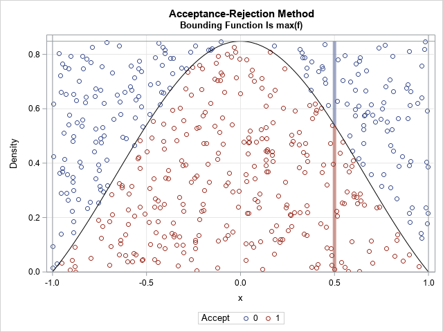
The following graph visualizes the acceptance-rejection method for this example. The values (x,y) are drawn uniformly at random from the bounding box [-1,1] x [0,max(f)]. For a given value of x, the probability that y is accepted is the ratio f(x) / max(f). The graph illustrates the probability that the variate x=0.5 is accepted. Notice that when x is near 0, the probability of acceptance is high; when x is near ±1, the probability is low.

Reformulating the simple acceptance-rejection method

The visualization of the algorithm reveals that many random (x,y) pairs in the bounding rectangle are not beneath the graph of the PDF and are therefore rejected. Only 59% of the potential variates are accepted. A more efficient simulation is one that accepts a greater proportion of the variates (ignoring the work required to generate the variates). For the Andrews PDF, we might use a triangle instead of a rectangle to construct a bounding region for the simulation.

This observation leads to the concept of an envelope function. In the previous section, the constant function h(x) = max(f) is used to generate the potential variates. This function is used for two reasons:

The function h is a scalar multiple of a density for a simple distribution. In this case, h(x) = max(f) is a multiple of the uniform density on [-1,1], and it is easy to generate variates from the uniform distribution.
The function h(x)=max(f) dominates the PDF in the sense that f(x) ≤ h(x) for all x in the domain.

Any function, h, that has these properties is called an envelope function. It is easy to satisfy the second condition, but harder to satisfy the first condition. The first condition means that you must consider only (scalar multiples of) density functions for distributions that have a simple algorithm for generating random variates. In this case, h(x) = M*U(x), where U is the PDF of the uniform distribution on [-1, 1] and M is a constant. You can perform a similar acceptance-rejection method if you use h(x) = M*g(x), where g is any PDF on [-1,1] for which you can easily generate random variates, provided that h dominates the Andrews PDF.

Using a triangular envelope function

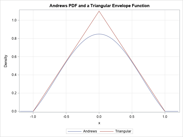
The PDF for the Andrews distribution is symmetric and unimodal. The simplest distribution that has this property is the triangular distribution on [-1,1], which has the PDF g(x) = 1 – |x|. You can define h(x) = M*g(x) to obtain an envelope function that dominates the Andrews PDF. The following graph overlays the Andrews PDF and the triangular envelope function for M=1.1:

Let's return to the simple acceptance-rejection method and slightly rewrite the algorithm. Notice that the random variate Y ~ U(0, max(f)) is used only to determine the acceptance or rejection of the point, x. Equivalently, for each x, you could generate a Bernoulli random variable with probability f(x)/max(f). That is, the IF-THEN statement in the SAS program could be rewritten as IF rand('Bernoulli', f/maxf) THEN ....

This reformulation generalizes to the case of a general envelope function. The following SAS DATA step implements a more sophisticated acceptance-rejection algorithm, which uses the triangular function to generates potential variates. The algorithm is as follows:

Generate a random variate, x, from the triangular distribution on [-1,1]. The RAND function in SAS generates triangular random variates on [0,1], so you need to apply the affine transformation x → 2*x-1 to obtain a variate on [-1,1].
Compute h(x) = M*g(x) where g(x)= 1 – |x| is the PDF of the triangular distribution on [-1,1]. To obtain a dominant function, you can set M=1.1.
Compute f(x) = (1/S) sin(πx)/(πx), which is the PDF of Andrews distribution on [-1,1].
Use the ratio f(x)/h(x) to determine the probability that x is accepted.
Repeat the process until you have accepted N variates. The result is a random sample of size N from the Andrews distribution.

The DATA step implementation is as follows:

/* Generate random variate from triangular distrib on [-1,1].
   Compute h(x) = M*PDF_{Triangle}(x) and 
           f(x) =   PDF_{Andrews}(x) and use the ratio
   f(x)/h(x) to determine the probability that x is accepted. */
data RandAndrewsTri;
S = 1.1789797;
M = 1.1;
call streaminit(1234);
pi = constant('pi');
numRand = 0;                        /* numRand = number of potential variates */
i = 0;                              /* i = number of accepted variates */
do while(i < &N);
   x = rand('Triangle', 0.5);       /* x ~ Tri(0,1) */
   x = 2*x - 1;                     /* transform so that x ~ Tri(-1, 1) */
   /* want h = M * pdf('Triangle', 0.5), but PDF doesn't support 'Triangle' */
   h = M*(1 - abs(x));
   numRand = numRand + 1;
   if x=0 then f = 1/S;
   else f = sin(pi*x) / (pi*x) / S;
   if rand('Bernoulli', f/h) then do; /* accept or reject according to f(x)/h(x) */
      i = i + 1;                    /* x is accepted; increment counter */
      output;
   end;
end;
keep x i numRand;
call symputx('AcceptFrac', round(&N / numRand, 0.0001));
run;
 
title "Random Sample from Andrews Distribution";
title2 "Candidates from Triangular Distribution";
title3 "Acceptance Rate = &AcceptFrac";
proc sgplot data=RandAndrewsTri;
   histogram x / scale=Percent;
   yaxis grid;
run;

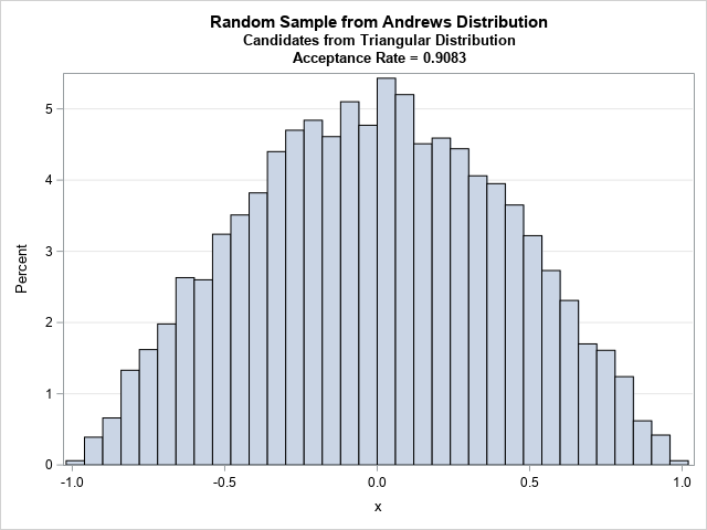
The histogram shows that the distribution of the random sample is similar in shape to the PDF of the Andrews distribution.

The efficiency of the envelope method

Using a triangular function as the envelope function improves the efficiency of the acceptance-rejection algorithm. If h(x) = M*g(x) is the triangular function on [-1,1] (where M=1.1 and g(x) is the triangular PDF), the area under the triangular function is 1.1. If you generate points uniformly at random in the triangle (bounded below by the X axis), the probability that a point is under the Andrews PDF is the ratio of areas: the area under the PDF divided by the area of the triangle. This ratio is 1 / 1.1 = 0.91. Thus, this acceptance-rejection algorithm should accept 91% of the candidate points, which is a substantial improvement over the 59% acceptance rate for the simpler algorithm.

The title of the histogram shows that the acceptance rate for the sample in this article is about 91%, in close agreement with theory.

Summary

One way to generate random samples from a distribution is to use an acceptance-rejection algorithm, which requires only the PDF of the distribution. A simple acceptance-rejection algorithm might have a low acceptance rate, which can make the algorithm inefficient for simulation studies that requires many samples. You can improve the efficiency by using an envelope function. An envelope function that dominates the PDF and is a scaled version of a density function of a distribution from which it is easy to generate random samples.

The example in this article has finite support, but you can construct similar envelope functions for distributions on infinite intervals such as [0, ∞) and (-∞, ∞).

Blogs