A SAS user asked how to interpret a rank-based correlation such as a Spearman correlation or a Kendall correlation. These are alternative measures to the usual Pearson product-moment correlation, which is widely used. The programmer knew that words like "weak," "moderate," and "strong" are sometimes used to describe the Pearson correlation according to certain cutpoints. For example, Schober, Boer, and Schwarte ("Correlation Coefficients: Appropriate Use and Interpretation," Anesthesia & Analgesia, 2018) suggest using the following cutpoints to associate sample correlations in medicine to clinical relevance:

• Negligible: the magnitude of the Pearson correlation is 0.0 - 0.09
• Weak: the magnitude of the Pearson correlation is 0.1 - 0.39
• Moderate: the magnitude of the Pearson correlation is 0.4 - 0.69
• Strong: the magnitude of the Pearson correlation is 0.7 - 0.89
• Very strong: the magnitude of the Pearson correlation is 0.9 - 1.0

The programmer asked whether there is a similar set of cutoff points for the Spearman or Kendall correlations. For many data sets, the answer is a qualified yes. This article shows how to create a set of cutoff points for the Spearman and Kendall correlations if the underlying data are bivariate normal. A simulation study shows that the same cutoff values are relevant for a certain class of non-normal data.

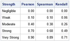
If you don't have time to read the full article, here are possible cutoff values for the rank-based correlation statistics, which are based on the recommendations for the Pearson correlation by Schober, Boer, and Schwarte (2018).

Expected relationships between correlations

Let's establish some notation. Given a data set, let r be the Pearson product-moment correlation, let s be the Spearman rank correlation, and let τ be the Kendall rank correlation. The definitions of these statistics are given in the SAS documentation for the CORR procedure. Kendall's τ is sometimes called "tau-b" to distinguish it from other definitions (called "tau-a" and "tau-c"). See a second article that compares the three definitions of Kendall's τ.

In general, you cannot convert between these statistics. I previously showed that the Pearson statistic is sensitive to extreme outliers. For example, you can add an outlier that will dramatically change the Pearson statistic but barely affect the rank-based statistics. Consequently, there is no formula that converts between a Pearson statistic and a rank-based statistic.

However, there is a difference between the letter of the law and the spirit of the law. In the case of an extreme outlier, you should not report the Pearson correlation, so it is meaningless to ask how to convert the statistic to one of the rank-based correlations. Similarly, if the data are not linearly related you should not use the Pearson statistic.

Many statistics (such as p-values) that are related to the Pearson correlation assume that the data are bivariate normal. Under that assumption, you can show that there is a well-defined relationship between the Pearson correlation and the rank-based correlations. For bivariate normal data, if R=E(r) is the expected value of the Pearson correlation, then

• S = 6/π arcsin(R/2) is the expected value of Spearman's correlation. Equivalently, R = 2 sin(π S/6).
• T = 2/π arcsin(R) is the expected value of Kendall's correlation. Equivalently, R = sin(π T /2).

The following SAS program displays the functions that convert between the expected values of the Pearson, Spearman, and Kendall statistics. The functions are plotted in red. A gray identity line is overlaid for reference.

/* Expected relationship between Pearson, Spearman, and Kendall correlations for bivariate normal data */
data PSFunc;
label Pearson = "Pearson (r)" Spearman = "Spearman (s)";
pi = constant('pi');
do Spearman = -1 to 1 by 0.05;
   Pearson = 2*sin(pi/6 * Spearman);
   output;
end;
run;
 
title "Pearson vs. Spearman Correlation";
title2 "Bivariate Normal Population";
proc sgplot data=PSFunc noautolegend;
   lineparm x=0 y=0 slope=1 / lineattrs=(color=lightgray);
   series x=Spearman y=Pearson / lineattrs=(color=red);
   xaxis grid; yaxis grid;
run;
 
data PKFunc;
label Pearson = "Pearson (r)" Kendall = "Kendall (tau)";
pi = constant('pi');
do Kendall = -1 to 1 by 0.05;
   Pearson = sin(pi/2 * Kendall);
   output;
end;
run;
 
title "Pearson vs. Kendall Correlation";
title2 "Bivariate Normal Population";
proc sgplot data=PKFunc noautolegend;
   lineparm x=0 y=0 slope=1 / lineattrs=(color=lightgray);
   series x=Kendall y=Pearson / lineattrs=(color=red);
   xaxis grid; yaxis grid;
run;

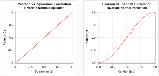
Notice that the function that converts between the Pearson and Spearman statistics is almost indistinguishable from the identity function! Recall that when |x| is small, then sin(x) ≈ x - x³ / 6. Therefore,
      2*sin(π S /6) ≈ π S/3 - (π³ / 648) S³ + ... ≈ 1.05 S - 0.05 S³ for S in [-1, 1].
This function differs from the identity function by only 2% on the interval [-1, 1]. Consequently, for bivariate normal data, the Pearson and Spearman statistics should be very close.

The function that converts between the Pearson and Kendall statistics is S-shaped. In general, the magnitude of the Kendall statistic for bivariate normal data is smaller than the Pearson statistic. For example, if the Pearson correlation for bivariate normal data is about 0.7, the Kendall statistic for the data is about 0.5.

The correlation statistics on bivariate normal data

The previous section shows results for the expected value of the Pearson and rank-based statistics for bivariate normal data. How do these relationships change for random samples of data? Let's run a simulation to find out. The following SAS IML program simulates 10 random samples from a bivariate normal distribution that has Pearson correlation ρ for multiple values of ρ. The statistics are computed on each sample. The call to PROC SGSCATTER displays the sample statistics against each other.

/* Test the theoretical results: generate 10 random bivariate normal samples of 
   size N=100 for each rho in (-0.95, 0.95) */
proc iml;
parm = do(-0.95, 0.95, 0.05); /* rho = {-0.95, -0.9, ..., 0.9, 0.95} */
mu = {0 0};
Cov = {1  .,                  /* matrix {1 rho, rho 1} */
       .  1};
N = 100;                      /* sample size */  
NRep = 10;                    /* number of samples for each rho value */
 
call randseed(12345);
create BiNormalCorr var {'rho' 'Group' 'Pearson' 'Spearman' 'Kendall'};
 
do i = 1 to ncol(parm);
   rho = parm[i];
   Cov[{2 3}] = rho;          /* replace off-diagonal elements */
   do Group = 1 to NRep;
      x = randnormal(N, mu, Cov);  /* X ~ bivariate normal from Pearson=rho */
      Pearson  = corr(x, "Pearson")[1,2];  /* compute the three statistics */
      Spearman = corr(x, "Spearman")[1,2];
      Kendall  = corr(x, "Kendall")[1,2];
      append;
   end;
end;
close;
quit;
 
title "Correlations for Bivariate Normal Data";
title2 "N = 100";
ods graphics / width=600px height=300px;
proc sgscatter data=BiNormalCorr;
   compare y=Pearson x=(Spearman Kendall) / colormodel=TwoColorRamp colorresponse=rho 
          markerattrs=(symbol=CircleFilled) grid; 
run;

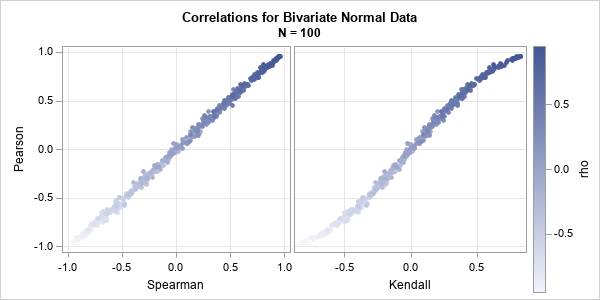
The graph shows that the estimates from these random bivariate normal samples are not far from the expected values for samples of size N=100.

The relationships for non-normal data

How do the relationships change for non-normal data? In general, that is an impossible question to answer. As explained earlier, extreme outliers can drastically change the Pearson statistic without changing the rank-based statistics by much. Therefore, there is no general formula that converts one statistic to another.

However, recall that the rank-based statistics are invariant under monotone increasing transformation. It is interesting, therefore, to ask how the relationships change if the bivariate normal data are transformed monotonically. The following SAS IML program repeats the previous simulation of bivariate normal data, but transforms the variables according to x1 → exp(x1); and x2 → sqrt(x2+8). The program computes the correlation statistics on the transformed data and plots the results:

/* repeat the simulation, but monotonically transform the x1 and x2 variables */
proc iml;
parm = do(-0.95, 0.95, 0.05); /* rho = {-0.95, -0.9, ..., 0.9, 0.95} */
mu = {0 0};
Cov = {1  .,                  /* matrix {1 rho, rho 1} */
       .  1};
N = 100;                      /* sample size */  
NRep = 10;                    /* number of samples for each rho value */
 
call randseed(12345);
create NonNormalCorr var {'rho' 'Group' 'PearsonZ' 'SpearmanZ' 'KendallZ'};
 
do i = 1 to ncol(parm);
   rho = parm[i];
   Cov[{2 3}] = rho;          /* replace off-diagonal elements */
   do Group = 1 to NRep;
      x = randnormal(N, mu, Cov);  /* X ~ bivariate normal from Pearson=rho */
      /* apply nonlinear monotone transforms such as EXP, SQRT, LOG, etc. */
      z1 = exp(x[,1]);
      z2 = sqrt(x[,2]+8);
      z = z1 || z2;
      PearsonZ  = corr(z, "Pearson")[1,2]; /* compute the three statistics */
      SpearmanZ = corr(z, "Spearman")[1,2];
      KendallZ  = corr(z, "Kendall")[1,2];
      append;
   end;
end;
close;
quit;
 
title "Correlations for Transformed Bivariate Normal Data";
title2 "x ==> exp(x); y ==> sqrt(y+8)";
proc sgscatter data=NonNormalCorr;
   compare y=PearsonZ x=(SpearmanZ KendallZ) / colormodel=TwoColorRamp colorresponse=rho 
          markerattrs=(symbol=CircleFilled) grid; 
run;

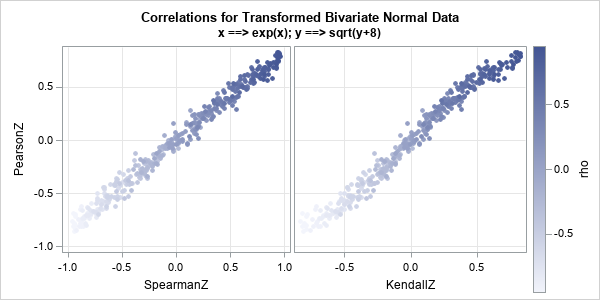
Although the data are transformed, the relationships between the statistics are still apparent. Again, the Pearson and Spearman statistics are approximately linearly related. The pairs of Pearson and Kendall statistics are modeled by an S-shaped function.

You can experiment with other monotone transformations. This behavior is fairly typical for the different (mostly tame) transformations that I tried. That is, the theoretical relationships for the expected value of the statistics are also apparent in these transformed samples. This suggests that if you want to bin the rank-based statistics into categories such as "weak," "moderate," and "strong," you could use the cutpoints for the Pearson statistic and convert them to cutpoints for the rank-based statistics by using the functions S = 6/π arcsin(R/2) and T = 2/π arcsin(R). These formulas were used to create the table at the beginning of this article, where R is the value in the Pearson column.

Summary

A researcher stated that categories such as "weak," "moderate," and "strong," are often assigned to certain values of the Pearson correlation. He wanted to know whether it is possible to map these categories to values of rank-based statistics such as Spearman's correlation and Kendall's association. In general, there is no formula that works for all data sets. However, this article shows that formulas do exist when the data are bivariate normal. Furthermore, a small simulation study suggests that the same relationships often are approximately valid when the variables are transformed by a monotonic transformation. Accordingly, if R is the Pearson statistic, the Spearman correlation is often approximated by 6/π arcsin(R/2). The Kendall statistic is often approximated by 2/π arcsin(R).