Why use rank correlation?

A previous article discusses rank correlation and lists some advantages of using rank correlation. However, the article does not show examples where an analyst might prefer to report the rank correlation instead of the traditional Pearson product-moment correlation. This article provides three examples where the rank correlation is a better measure of association than the Pearson correlation. I will use the Spearman correlation as an example of a rank-based correlation, but the examples also apply to other rank-based statistics, such as Kendall's correlation.

The examples correspond to following three advantages of rank-based correlation:

Rank correlation is robust to outliers.
Rank correlation can reveal nonlinear relationships.
Rank correlation is invariant under monotone increasing transformations.

Rank correlation is robust to outliers

The primary reason to use rank correlation is that it is robust to outliers. The traditional Pearson correlation uses sample moments of the data (means and standard deviations) to estimate the linear association between two variables. But means and standard deviations are not robust statistics; they are influenced by extreme outliers.

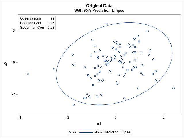
Consider the following sample of N=99 observations. The data are generated from a bivariate normal model for which the (Pearson) correlation is 0.3. You can use the PEARSON and SPEARMAN options in PROC CORR in SAS to show that the Pearson and Spearman estimates are both close to the population value. The Pearson estimate is r = 0.26 and the Spearman estimate is s = 0.28. You can also ask PROC CORR to create a scatter plot of the data and to include a 95% prediction ellipse for new observations. The ellipse assumes that the data are bivariate normal.

data Sample;
input x1 x2 @@;
datalines;
. . 0.82 -0.28 1.54 -0.71 -0.14 0.95 0.07 1.19 -0.15 0.23 -1.15 -0.81 -0.45 0.13 -0.22 0.14 -0.42 0.11 
0.91 1.69 1.66 -1.11 -0.76 0.37 1.43 0.77 -0.02 0.44 0.74 -0.31 1.37 0.49 -1.31 -2.24 0.6 0.96 1.05 -0.64 
1.08 -0.15 -1.16 -0.79 0.94 -1.6 -0.43 -0.08 -1.04 0.44 0.39 -0.63 -0.07 1.32 0.78 1.5 0.33 0.01 1.14 -0.78 
0.35 -0.86 0.15 0.7 -0.59 -1.17 -0.03 0.23 -0.6 -2.01 0.06 -1.21 0.77 1.51 -0.87 -0.34 0.05 -1.31 0.72 0.64 
0.17 1.19 0.21 0.02 -0.76 0.28 0.68 -0.46 -1.27 -2.21 2.4 -1.61 -0.39 0.37 -0.68 0.76 -0.75 -0.21 0.3 -0.26 
-0.77 -0.71 -1.77 -0.12 -0.87 1.08 -0.21 0.27 0.7 1.11 0.59 0.05 0.13 -0.78 -0.33 0 -1.76 -2.65 -0.36 -0.16 
1.33 1.98 0.53 1.14 0.35 -2.23 -0.71 -1.11 0.2 0.38 0.81 0.16 -0.66 -0.58 0.35 0.47 0.8 0.98 -2.57 -0.41 
0.96 1.35 0.48 -0.46 1.05 0.64 -0.26 -0.55 -0.87 -0.84 0.16 0.98 0.41 0.6 -1.8 0.5 -1.3 -0.29 -0.98 1.44 
0.2 -0.02 -0.95 -1.41 0.8 0.66 -0.6 -0.3 -0.32 0.08 0.15 0.07 -0.54 -1.09 -0.53 0.42 0.04 1.27 -0.86 0.67 
0.24 0.2 1.56 0.21 0.01 0.84 -1.11 -2.13 -0.78 -2.12 -1.05 -0.98 -3.68 -0.72 -1.2 -1.97 1.66 -0.53 -0.39 2.43 
;
 
title "Original Data";
proc corr data=Sample noprob nosimple Pearson Spearman plot=scatter;
   var x1 x2;
run;

Now, let's add an extreme outlier. Specifically, add a new observation at x1=10 for which x2 is extremely large (or extremely small). If you add the outlier and recompute the Pearson and Spearman correlations, you will discover that the Pearson correlation has changed by a lot, whereas the Spearman rank-based correlation has changed by only a little. The following SAS DATA step adds the outlier (10, -50) to the data.

title "Extreme Leverage Point: Low Value";
data SampleOut1;
set Sample;
if _N_=1 then do;
   x1 = 10;  x2 = -50;
end;
proc corr data=SampleOut1 noprob nosimple Pearson Spearman;
   var x1 x2;
run;

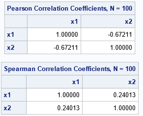
Notice that by adding one outlier, the Pearson correlation has decreased from +0.26 to -0.67! In contrast, the Spearman correlation barely changed from 0.28 to 0.24. You can perform a similar experiment by adding an outlier that has an extremely large value for x2. For the next example, the outlier is the point (10, +50):

title "Extreme Leverage Point: High Value";
data SampleOut2;
set Sample;
if _N_=1 then do;
   x1 = 10;  x2 = 50;
end;
proc corr data=SampleOut2 noprob nosimple Pearson Spearman;
   var x1 x2;
run;

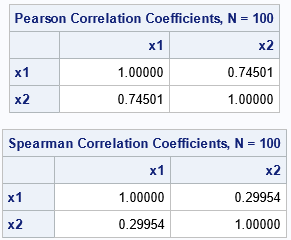
Again, the Pearson correlation has changed dramatically (from 0.26 to 0.75) whereas the Spearman correlation has barely changed (from 0.28 to 0.30). These examples show that the Pearson correlation is highly influenced by an extreme outlier whereas the Spearman correlation is not.

Rank correlation captures nonlinear relationships

A second reason that people use a rank-based correlation is that the Pearson correlation measures the strength of a linear relationship, whereas the Spearman correlation can be used for some nonlinear relationships. The next example measures the association between the MPG_City and Weight variables for 428 vehicles in the Sashelp.cars data set. The following call to PROC CORR displays the Pearson and Spearman statistics:

title "Nonlinear Relationship";
proc corr data=Sashelp.Cars noprob nosimple plot=scatter Pearson Spearman;
   var MPG_City Weight;
run;

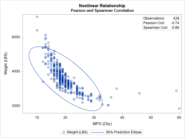
The procedure reports that the sample Pearson statistic is -0.74. In contrast, the Spearman correlation is -0.86, which is larger in magnitude. The Pearson statistic measures the linear relationship between the variables. However, the scatter plot reveals that the variables are not, in fact, linearly related. The larger magnitude for the Spearman statistic is perhaps a better indication that small (respectively, large) values of MPG_City are strongly associated with small (respectively, large) values of Weight.

Rank correlation is invariant under monotone increasing transformations

Another reason to use a rank-based correlation is if you need to transform one or more variables. Recall that a rank-based statistic is invariant under any monotone increasing transformation of the data because the ranks themselves are unchanged under the transformation. Thus, you can report the Spearman correlation for transformed data, and the readers know that the Spearman correlation for the original data are the same values.

To give an example, suppose you want to perform a Box-Cox transform of the MPG_City and Weight variables. The following DATA step implements the following monotone transformations of the original variables:

Transform the MPG_City variable by using the power transformation x → (x^λ -1) / λ, where λ = -0.5.
Transform the Weight variable by using the logarithmic transformation x → log(x).

Every Box-Cox transformation is monotone increasing. Because the Spearman correlation is invariant under any monotone increasing transformation, the Spearman correlation for the transformed variables is unchanged from the Spearman correlation of the original variables.

title "Original Correlations";
proc corr data=Sashelp.Cars noprob nosimple Pearson Spearman;
   label MPG_City= Weight=;
   var MPG_City Weight;
run;
 
title "Correlations between Transformed Variables";
data C;
set Sashelp.Cars;
lambda = -0.5;
xformMPG = (MPG_City**lambda -1) / lambda;
logWeight = log(Weight);
run;
 
proc corr data=C noprob nosimple Pearson Spearman plots=scatter;
   var xformMPG logWeight;
run;

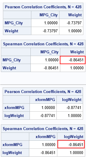
As predicted, the Spearman correlation between the transformed variables is identical to the original Spearman correlation. The Pearson correlation does not have that property. The Pearson correlation is invariant only under linear transformations.

Summary

A previous article discusses rank correlation and lists some advantages of using rank correlation. This article provides examples of some of the advantages. Specifically, this article shows that a rank-based correlation is resistant to extreme outliers, can measure the association between (some) nonlinearly related variables, and is invariant under any monotone increasing transformation, such as a Box-Cox transformation.

Blogs