A SAS programmer wanted to compute the distribution of X-Y, where X and Y are two beta-distributed random variables. Pham-Gia and Turkkan (1993) derive a formula for the PDF of this distribution. Unfortunately, the PDF involves evaluating a two-dimensional generalized hypergeometric function, which is not available in all programming languages. Hypergeometric functions are not supported natively in SAS, but this article shows how to evaluate the generalized hypergeometric function for a range of parameter values. By using the generalized hypergeometric function, you can evaluate the PDF of the difference between two beta-distributed variables.
The difference between two beta random variables
Before doing any computations, let's visualize what we are trying to compute. Let X ~ Beta(a1, b1) and Y ~ Beta(a1, b1) be two beta-distributed random variables. We want to determine the distribution of the quantity d = X-Y. One way to approach this problem is by using simulation: Simulate random variates X and Y, compute the quantity X-Y, and plot a histogram of the distribution of d. Because each beta variable has values in the interval (0, 1), the difference has values in the interval (-1, 1).
The following simulation generates 100,000 pairs of beta variates: X ~ Beta(0.5, 0.5) and Y ~ Beta(1, 1). Both X and Y are U-shaped on (0,1). The following simulation generates the differences, and the histogram visualizes the distribution of d = X-Y:
/* Case 2 from Pham-Gia and Turkkan, 1993, p. 1765 */ %let a1 = 0.5; %let b1 = 0.5; %let a2 = 1; %let b2 = 1; %let N = 1E5; data BetaDiff; call streaminit(123); do i = 1 to &N; x = rand("beta", &a1, &b1); y = rand("beta", &a2, &b2); d = x - y; output; end; drop i; run; title "Distribution of X-Y"; title2 "X~beta(&a1,&b1); Y~beta(&a2,&b2)"; proc sgplot data=BetaDiff; histogram d; run; |
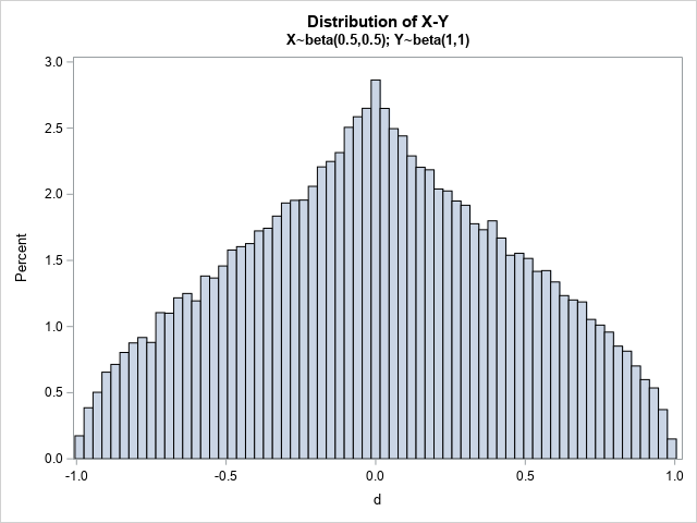
For these values of the beta parameters, the distribution of the differences between the two beta variables looks like an "onion dome" that tops many Russian Orthodox churches in Ukraine and Russia. For other choices of parameters, the distribution can look quite different. The remainder of this article defines the PDF for the distribution of the differences. The formula for the PDF requires evaluating a two-dimensional generalized hypergeometric distribution.
Appell's hypergeometric function
A previous article discusses Gauss's hypergeometric function, which is a one-dimensional function that has three parameters. For certain parameter
values, you can compute Gauss's hypergeometric function by computing a definite integral.
The two-dimensional generalized hypergeometric function that is used by Pham-Gia and Turkkan (1993),
is called Appell's hypergeometric function (denoted F1 by mathematicians).
Appell's function can be evaluated by solving a definite integral that looks very similar to the integral encountered in evaluating the 1-D function. Appell's F1 contains four parameters (a,b1,b2,c) and two variables (x,y). In statistical applications, the variables and parameters are real-valued.
For the parameter values c > a > 0, Appell's F1 function can be evaluated by computing the following integral:
\(F_{1}(a,b_{1},b_{2},c;x,y)={\frac {1}{B(a, c-a)}} \int _{0}^{1}u^{a-1}(1-u)^{c-a-1}(1-x u)^{-b_{1}}(1-y u)^{-b_{2}}\,du\)
where B(s,t) is the complete beta function, which is available in SAS by using the BETA function. Both arguments to the BETA function must be positive, so evaluating the BETA function requires that c > a > 0. Notice that the integration variable, u, does not appear in the answer.
Appell's hypergeometric function is defined for |x| < 1 and |y| < 1. Notice that the integrand is unbounded when
either x → 1 or y → 1 (assuming b1 > 0 and b2 > 0).
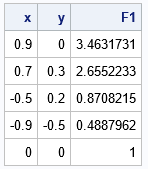
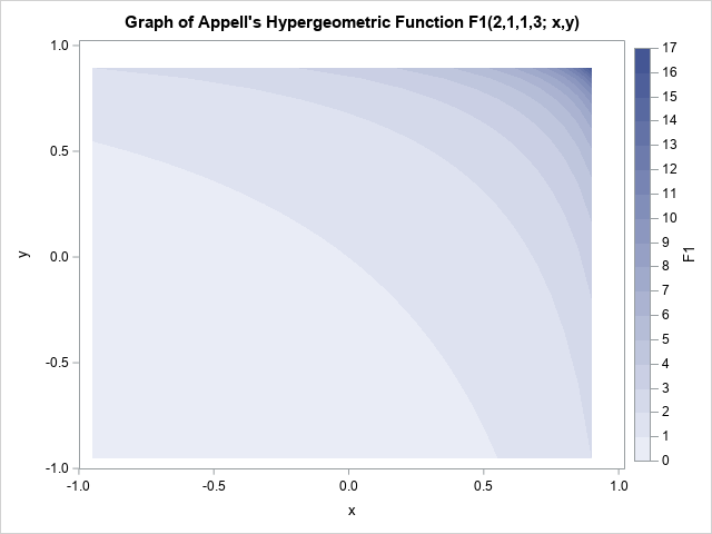
The following SAS IML program defines a function that uses the QUAD function to evaluate the definite integral, thereby evaluating Appell's hypergeometric function for the parameters (a,b1,b2,c) = (2,1,1,3). A table shows the values of the function at a few (x,y) points. The graph shows a contour plot of the function evaluated on the region [-0.95, 0.9] x [-0.95, 0.9].
/* Appell hypergeometric function of 2 vars F1(a,b1,b2; c; x,y) is a function of (x,y) with parms = a // b1 // b2 // c; F1 is defined on the domain {(x,y) | |x|<1 and |y|<1}. You can evaluate F1 by using an integral for c > a > 0, as shown at https://en.wikipedia.org/wiki/Appell_series#Integral_representations */ proc iml; /* Integrand for the QUAD function */ start F1Integ(u) global(g_parm, g_x, g_y); a=g_parm[1]; b1=g_parm[2]; b2=g_parm[3]; c=g_parm[4]; x=g_x; y=g_y; numer = u##(a-1) # (1-u)##(c-a-1); denom = (1-u#x)##b1 # (1-u#y)##b2; return( numer / denom ); finish; /* Evaluate the Appell F1 hypergeometric function when c > a > 0 and |x|<1 and |y|<1 Pass in parm = {a, b1, b2, c} and z = (x1 y1, x2 y2, ... xn yn}; */ start AppellF1(z, parm) global(g_parm, g_x, g_y); /* transfer parameters to global symbols */ g_parm = parm; a = parm[1]; b1 = parm[2]; b2 = parm[3]; c = parm[4]; n = nrow(z); F = j(n, 1, .); if a <= 0 | c <= a then do; /* print error message or use PrintToLOg function: https://blogs.sas.com/content/iml/2023/01/25/printtolog-iml.html */ print "This implementation of the F1 function requires c > a > 0.", parm[r={'a','b1','b2','c'}]; return( F ); end; /* loop over the (x,y) values */ do i = 1 to n; /* defined only when |x| < 1 */ g_x = z[i,1]; g_y = z[i,2]; if g_x^=. & g_y^=. & abs(g_x)<1 & abs(g_y)<1 then do; call quad(val, "F1Integ", {0 1}) MSG="NO"; F[i] = val; end; end; return( F / Beta(a, c-a) ); /* scale the integral */ finish; /* Example of calling AppellF1 */ parm = {2, 1, 1, 3}; parm = {2, 1, 1, 3}; xy = { 0.9 0, 0.7 0.3, -0.5 0.2, -0.9 -0.5, 0 0}; F1 = AppellF1(xy, parm); print xy[L="" c={'x' 'y'}] F1; |
The PDF of beta differences
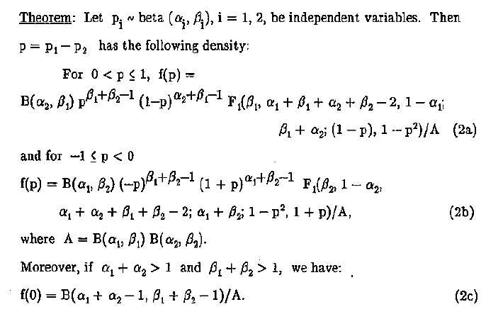
Pham-Gia and Turkkan (1993) derive the PDF of the distribution for the difference between two beta random variables, X ~ Beta(a1,b1) and Y ~ Beta(a2,b2). The PDF is defined piecewise. There are different formulas, depending on whether the difference, d, is negative, zero, or positive. The formulas use powers of d, (1-d), (1-d2), the Appell hypergeometric function, and the complete beta function. The formulas are specified in the following program, which computes the PDF. Notice that linear combinations of the beta parameters are used to construct the parameters for Appell's hypergeometric function.
/* Use Appell's hypergeometric function to evaluate the PDF of the distribution of the difference X-Y between X ~ Beta(a1,b1) and Y ~ Beta(a2,b2) */ start PDFBetaDiff(_d, _parm); a1=_parm[1]; b1=_parm[2]; a2=_parm[3]; b2=_parm[4]; n = nrow(_d)*ncol(_d); PDF = j(n, 1, .); if a1<=0 | b1<=0 | a2<=0 | b2<=0 then do; print "All parameters must be positive", a1 b1 a2 b2; return(PDF); end; A = Beta(a1,b1) * Beta(a2,b2); do i = 1 to n; d = _d[i]; *print d a1 b1 a2 b2; if d = . then PDF[i] = .; if abs(d) < 1 then do; /* Formulas from Pham-Gia and Turkkan, 1993 */ if abs(d)<1e-14 then do; if a1+a2 > 1 & b1+b2 > 1 then PDF[i] = Beta(a1+a2-1, b1+b2-1) / A; *print "d=0" (a1+a2-1)[L='a1+a2-1'] (b1+b2-1)[L='b1+b2-1'] (PDF[i])[L='PDF']; end; else if d > 0 then do; /* (0,1] */ parm = b1 // a1+b1+a2+b2-2 // 1-a1 // a2+b1; xy = 1-d || 1-d##2; F1 = AppellF1(xy, parm); PDF[i] = Beta(a2,b1) # d##(b1+b2-1) # (1-d)##(a2+b1-1) # F1 / A; *print "d>0" xy (PDF[i])[L='PDF']; end; else do; /* [-1,0) */ parm = b2 // 1-a2 // a1+b1+a2+b2-2 // a1+b2; xy = 1-d##2 || 1+d; F1 = AppellF1(xy, parm); PDF[i] = Beta(a1,b2) # (-d)##(b1+b2-1) # (1+d)##(a1+b2-1) # F1 / A; *print "d<0" xy (PDF[i])[L='PDF']; end; end; end; return PDF; finish; print "*** Case 2 in Pham-Gia and Turkkan, p. 1767 ***"; a1 = 0.5; b1 = 0.5; a2 = 1; b2 = 1; parm = a1//b1//a2//b2; d = {-0.9, -0.5, -0.25, 0, 0.25, 0.5, 0.9}; PDF = PDFBetaDiff(d, parm); print d PDF; |
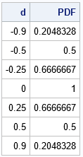
Notice that the parameters are the same as in the simulation earlier in this article. The following graph visualizes the PDF on the interval (-1, 1):
/* graph the distribution of the difference */ d = T(do(-0.975, 0.975, 0.025)); PDF = PDFBetaDiff(d, parm); title "X-Y for X ~ Beta(0.5,0.5) and Y ~ Beta(1,1)"; title2 "Fig 1, p. 1766"; call series(d, PDF) grid={x y}; |
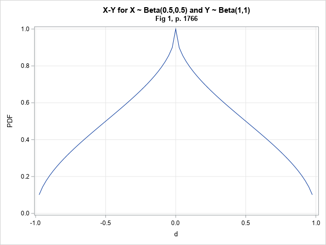
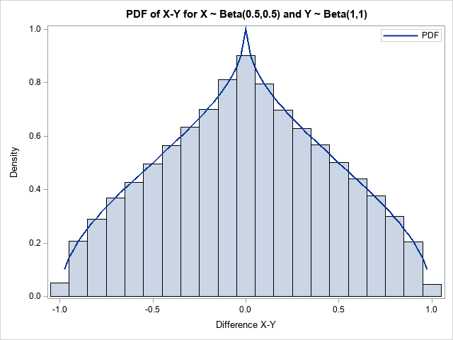
The PDF, which is defined piecewise, shows the "onion dome" shape that was noticed for the distribution of the simulated data. The following graph overlays the PDF and the histogram to confirm that the two graphs agree.
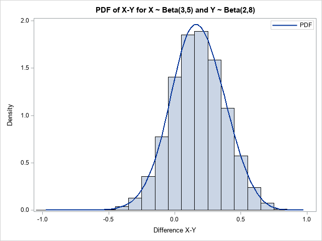
Not every combination of beta parameters results in a non-smooth PDF. For example, if you define X ~ beta(3,5) and Y ~ beta(2, 8), then you can compute the PDF of the difference, d = X-Y, by changing the parameters as follows:
/* Case 5 from Pham-Gia and Turkkan, 1993, p. 1767 */ a1 = 3; b1 = 5; a2 = 2; b2 = 8; parm = a1//b1//a2//b2; |
If you rerun the simulation and overlay the PDF for these parameters, you obtain the following graph:
Summary
The distribution of X-Y, where X and Y are two beta-distributed random variables, has an explicit formula (Pham-Gia and Turkkan, 1993). Unfortunately, the PDF involves evaluating a two-dimensional generalized hypergeometric function, which is a complicated special function. Hypergeometric functions are not supported natively in SAS, but this article shows how to evaluate the generalized hypergeometric function for a range of parameter values, which enables you to evaluate the PDF of the difference between two beta-distributed variables.
You can download the following SAS programs, which generate the tables and graphs in this article:
- How to compute Appell's hypergeometric function in SAS
- How to compute the PDF of the difference between two beta-distributed variables in SAS
References
- T. Pham-Gia and N. Turkkan (1993) "Bayesian analysis of the difference of two proportions," Communications in Statistics - Theory and Methods, 22(6), 1755-1771.
- The formula for the PDF, scanned from Pham-Gia and Turkkan (1993).
- Weisstein, Eric W. "Appell Hypergeometric Function." From MathWorld--A Wolfram Web Resource.
