A previous article discusses the definitions of three kinds of moments for a continuous probability distribution: raw moments, central moments, and standardized moments. These are defined in terms of integrals over the support of the distribution. Moments are connected to the familiar shape features of a distribution: the mean, variance, skewness, and kurtosis. This article shows how to evaluate integrals in SAS to evaluate the moments of a continuous distribution, and how to compute the mean, variance, skewness, and kurtosis of the distribution.

Notice that this article is not about how to compute the sample estimates. You can easily use PROC MEANS or PROC UNIVARIATE to compute the sample mean, sample variance, and so forth, from data. Rather, this article is about how to compute the quantities for the probability distribution.

Definitions of moments of a continuous distribution

Evaluating a moment requires performing an integral. The domain of integration is the support of the distribution. This is often infinite (for example, the normal distribution on (-∞, ∞)) or semi-bounded (for example, the lognormal distribution on [0,∞)), but sometimes it is finite (for example, the beta distribution on [0,1]). The QUAD subroutine in SAS/IML software can compute integrals on finite, semi-infinite, and infinite domains. You need to specify a SAS/IML module that evaluates the integrand at an arbitrary point in the domain. To compute a raw moment, the integrand is computed as the product of x and the probability density function (PDF). To compute a central moment, the integrand is the product the PDF and a power of (x - μ), where μ is the mean of the distribution. Let f(x) be the PDF. The moments relate to the mean, variance, skewness, and kurtosis as follows:

• The mean is the first raw moment: $\mu = \int_{-\infty}^{\infty} x f(x)\, dx$
• The variance is the second central moment: $\sigma^2 = \int_{-\infty}^{\infty} (x - \mu)^2 f(x)\, dx$
• The skewness is the third standardized moment: $\mu_3 / \sigma^3$ where $\mu_3 = \int_{-\infty}^{\infty} (x - \mu)^3 f(x)\, dx$ is the third central moment.
• The full kurtosis is the fourth standardized moment: $\mu_4 / \sigma^4$ where $\mu_4 = \int_{-\infty}^{\infty} (x - \mu)^4 f(x)\, dx$ is the fourth central moment. For consistency with the sample estimates, you can compute the excess kurtosis by subtracting 3 from this quantity.

Compute moments in SAS

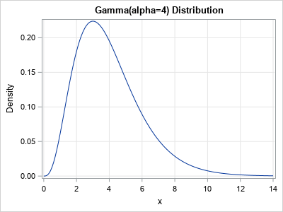
To demonstrate how to compute the moments of a continuous distribution, let's use the gamma distribution with shape parameter α=4. The PDF of the Gamma(4) distribution is shown to the right. The domain of the PDF is [0, ∞). The mean, variance, skewness, and excess kurtosis for the gamma distribution can be computed analytically. The formulas are given in the Wikipedia article about the gamma distribution. The following SAS/IML program evaluates the formulas for α=4.

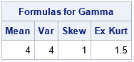
/* compute moments (raw, central, and standardized) for a probability distribution */
proc iml;
/* Formulas for the mean, variance, skewness, and excess kurtosis, 
   of the gamma(alpha=4) distribution from https://en.wikipedia.org/wiki/Gamma_distribution
*/
alpha = 4;                 /* shape parameter */
mean  = alpha;             /* mean */
var   = alpha;             /* variance */
skew  = 2 / sqrt(alpha);   /* skewness */
exKurt= 6 / alpha;         /* excess kurtosis */
colNames = {'Mean' 'Var' 'Skew' 'Ex Kurt'};
print (mean||var||skew||exKurt)[c=colNames L="Formulas for Gamma"];

Let's evaluate these same quantities by performing numerical integration of the integrals that define the moments of the distribution:

/* return the PDF of a specified probability distribution */
start f(x) global(alpha);
   return  pdf("Gamma", x, alpha);  /* return the PDF evaluated at x */
finish;
 
/* the first raw moment is the mean: \int x*f(x) dx */
start Raw1(x);
   return( x # f(x) );              /* integrand for first raw moment */
finish;
 
/* the second central moment is the variance: \int (x-mu)^2*f(x) dx */
start Central2(x) global(mu);
   return( (x-mu)##2 # f(x) );      /* integrand for second central moment */
finish;
 
/* the third central moment is the UNSTANDARDIZE skewness: \int (x-mu)^3*f(x) dx */
start Central3(x) global(mu);
   return( (x-mu)##3 # f(x) );      /* integrand for third central moment */
finish;
 
/* the fourth central moment is the UNSTANDARDIZE full kurtosis: \int (x-mu)^4*f(x) dx */
start Central4(x) global(mu);
   return( (x-mu)##4 # f(x) );      /* integrand for fourth central moment */
finish;
 
Interval = {0, .I};                 /* support of gamma distribution is [0, infinity) */
call quad(mu, "Raw1", Interval);    /* define mu, which is used for central moments */
call quad(var, "Central2", Interval);
call quad(cm3, "Central3", Interval);
call quad(cm4, "Central4", Interval);
 
/* do the numerical calculations match the formulas? */
skew = cm3 / sqrt(var)##3;          /* standardize 3rd central moment */
exKurt = cm4 / sqrt(var)##4 - 3;    /* standardize 4th standard moment; subtract 3 to get excess kurtosis */
print (mu||var||skew||exKurt)[c=colNames L="Numerical Computations for Gamma"];

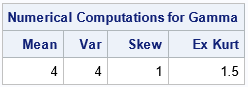
For this distribution, the numerical integration produces numbers that exactly match the formulas. For other distributions, the numerical integration might differ from the exact values by a tiny amount.

Checking the moments against the sample estimates

Not all distributions have analytical formulas for the mean, variance, and so forth. When I compute a new quantity, I like to verify the computation by comparing it to another computation. In this case, you can compare the distributional values to the corresponding sample estimates for a large random sample. In other words, if you generate a large random sample from the Gamma(4) distribution and compute the sample mean, sample, variance, and so forth, you should obtain sample estimates that are close to the corresponding values for the distribution. You can perform this simulation in the DATA step or in the SAS/IML language. The following statements use the DATA step and PROC MEANS to generate a random sample of size N=10,000 from the gamma distribution:

data Gamma(keep = x);
alpha = 4;
call streaminit(1234);
do i = 1 to 10000;
   x = rand("Gamma", alpha);
   output;
end;
run;
 
proc means data=Gamma mean var skew kurt NDEC=3;
run;

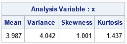
As expected, the sample estimates are close to the values of the distribution. The sample skewness and kurtosis are biased statistics and have relatively large standard errors, so the estimates for those parameters might not be very close to the distributional values, even for a large sample.

Summary

This article shows how to use the QUAD subroutine in SAS/IML software to compute raw and central moments of a probability distribution. This article uses the gamma distribution with shape parameter α=4, but the computation generalizes to other distributions. The important step is to write a user-defined function that evaluates the PDF of the distribution of interest. For many common distributions, you can use the PDF function in Base SAS to evaluate the density function. You also must specify the support of the distribution, which is often an infinite or semi-infinite domain of integration. When the moments exist, you can compute the mean, variance, skewness, and kurtosis of any distribution.