I've previously shown how to use Monte Carlo simulation to estimate probabilities and areas. I illustrated the Monte Carlo method by estimating π ≈ 3.14159... by generating points uniformly at random in a unit square and computing the proportion of those points that were inside the unit circle. The previous article used the SAS/IML language to estimate the area. However, you can also perform a Monte Carlo computation by using the SAS DATA step. Furthermore, the method is not restricted to simple geometric shapes like circles. You can use the Monte Carlo technique to estimate the area of any bounded planar figure. You merely need a bounding box and a way to assess whether a random point is inside the figure. This article uses Monte Carlo simulation to estimate the area of a polar rose with five petals.

The polar rose

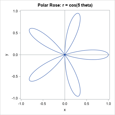
You can read about how to draw a polar rose in SAS. The simplest form of the polar rose is given by the polar equation r = cos(k θ), where k is an integer, r is the polar radius, and θ is the polar angle (0 ≤ θ ≤ 2 π).

The following DATA step computes the coordinates of the polar rose for k=5. The subsequent call to PROC SGPLOT graphs the curve.

%let k = 5;      /* for odd k, the rose has k petals */
/* draw the curve r=cos(k * theta) in polar coordinates:
   https://blogs.sas.com/content/iml/2015/12/16/polar-rose.html */
data Rose;
do theta = 0 to 2*constant("pi") by 0.01;
   r = cos(&k * theta);       /* rose */
   x = r*cos(theta);          /* convert to Euclidean coordinates */
   y = r*sin(theta);
   output;
end;
keep x y;
run;
 
title "Polar Rose: r = cos(&k theta)";
ods graphics / width=400px height=400px;
proc sgplot data=Rose aspect=1;
   refline 0 / axis=x;   refline 0 / axis=y;
   series x=x y=y;
   xaxis min=-1 max=1;   yaxis min=-1 max=1;
run;

The remainder of this article uses Monte Carlo simulation to estimate the area of the five-petaled rose. The answer is well-known and is often proved in a calculus class. When k is odd, the area of the rose generated by r = cos(k θ) is A = π / 4 ≈ 0.7854.

Monte Carlo estimates of area

To estimate the area of a geometric figure by using Monte Carlo simulation, do the following:

1. Generate N points uniformly in a bounding rectangle.
2. For each point, compute whether the point is inside the figure. This enables you to form the proportion, p, of points that are inside the figure.
3. Estimate the area of the figure as p A_R, where A_R is the area of the bounding rectangle.
4. Optionally, you can construct a confidence interval for the area. A confidence interval for the binomial proportion is p ± z_α sqrt(p(1-p) / N), where z_α is the 1-α/2 quantile of the normal distribution. If you multiply the interval by A_R, you get a confidence interval for the area.

The Monte Carlo method produces a simulation-based estimate. The answer depends on the random number stream, so you obtain AN estimate rather than THE estimate. In this article, the rose will be bounded by using the rectangle [-1, 1] x [-1, 1], which has area A_R = 4.

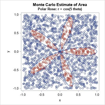
The plot to the right shows the idea of a Monte Carlo estimate. The plot shows 3,000 points from the uniform distribution on the rectangle [-1, 1] x [-1, 1]. There are 600 points, shown in red, that are inside one of the petals of the polar rose. Because 600 is 20% of the total number of points, we estimate that the rose occupies 20% of the area of the square. Thus, with N=3000, an estimate of the area of the rose is 0.2*A_R = 0.8, which is somewhat close to π / 4 ≈ 0.7854.

Statistical theory suggests that the accuracy of the proportion estimate should be proportional to 1/sqrt(N). This statement has two implications:

1. If you want to double the accuracy of an estimate, you must increase the number of simulated points fourfold.
2. Loosely speaking, if you use one million points (N=1E6), you can expect your estimate of the proportion to be roughly 1/sqrt(N) = 1E-3 units from the true proportion. A later section makes this statement more precise.

A Monte Carlo implementation in the SAS DATA step

Let's increase the number of simulated points to improve the accuracy of the estimates. We will use one million (1E6) random points in the bounding rectangle.

There are two primary ways to obtain the Monte Carlo estimate. The first way is to generate a data set that has N random points and contains a binary indicator variable that specifies whether each point is inside the figure. You can then use PROC FREQ to obtain an estimate of the binomial proportion and a confidence interval for the proportion, as follows:

%let N = 1E6;           /* generate N random points in bounding rectangle */
data Area;
/* define rectangle on which to uniformly sample */
a = -1;  b = 1;         /* x in (a,b) */
c = -1;  d = 1;         /* y in (a,b) */
AreaRect = (b-a)*(d-c); /* area of bounding rectangle */
call streaminit(12345);
do i = 1 to &N;
   x = rand("Uniform", a, b);
   y = rand("Uniform", c, d);
   /* Add code HERE to determine if (x,y) is inside the region of interest */
   theta = atan2(y, x);                 /* notice order */
   rxy = sqrt(x**2 + y**2);             /* observed value of r */
   isInside = (rxy < cos(&k * theta));  /* inside the rose */
   output;
end;
keep x y isInside;
run;
 
/* isInside is binary, so can compute binomial CI for estimate */
proc freq data=Area;
   tables IsInside / binomial(level='1' CL=wald);   /* Optional: Use BINOMIAL option for CL */
   ods select Binomial BinomialCLs;
run;

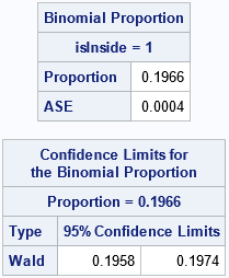
The proportion of points inside the figure is 0.1966. A 95% confidence interval for the proportion is [0.1958, 0.1974]. To transform these values into areas, you need to multiply them by the area of the bounding rectangle, which is 4. Thus, an estimate for the area of the rose is 0.7864, and a confidence interval is [0.7832, 0.7896]. This estimate is within 0.001 units of the true area, which is π/4 ≈ 0.7854. If you change the random number seed, you will get a different estimate.

Manual computation of binomial estimates

If you are comfortable with programming the binomial proportion yourself, you can perform the entire computation inside a DATA step without using PROC FREQ. The advantage of this method is that you do not generate a data set that has N observations. Rather, you can count the number of random points that are inside the rose, and merely output an estimate of that area and a confidence interval. By using this method, you can simulate millions or billions of random points without writing a large data set. The following DATA step demonstrates this technique:

%let N = 1E6;   
data MCArea;
/* define rectangle on which to uniformly sample */
a = -1;  b = 1;         /* x in (a,b) */
c = -1;  d = 1;         /* y in (a,b) */
AreaRect = (b-a)*(d-c); /* area of bounding rectangle */
call streaminit(12345);
do i = 1 to &N;
   x = rand("Uniform", a, b);
   y = rand("Uniform", c, d);
   /* Add code HERE to determine if (x,y) is inside the region of interest */
   theta = atan2(y, x);                 /* notice order */
   rxy = sqrt(x**2 + y**2);             /* observed value of r */
   isInside = (rxy < cos(&k * theta));  /* inside the rose */
   /* we now have binary variable isInside */
   sumInside + isInside;                /* count the number of points inside */
end;
 
/* simulation complete; output only the results */
p = sumInside / &N;                     /* proportion of points inside region */
AreaEst = p * AreaRect;                 /* estimate of area of the figure */
/* Optional: Since p is a binomial proportion, you can get a confidence interval */
alpha = 0.05;
zAlpha = quantile("Normal", 1-alpha/2);  /* = 1.96 when alpha=0.05 */
SE = zAlpha*sqrt(p*(1-p)/&N);
LCL = (p - SE)*AreaRect;
UCL = (p + SE)*AreaRect;
/* Optional: if you know the true area, you can compare it with MC estimate */
ExactArea = constant('pi') / 4;    
Difference = ExactArea - AreaEst;
keep AreaRect p AreaEst LCL UCL ExactArea Difference;
label AreaRect="Area of Rectangle" p = "Proportion Inside" AreaEst="MC Area Estimate" 
      ExactArea="Exact Area" LCL="95% Lower Limit" UCL="95% Upper Limit";
run;
 
proc print data=MCArea noobs label; 
   format Difference 8.5;
run;

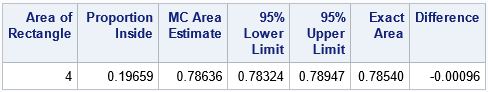
Notice that this DATA step outputs only one observation, whereas the previous DATA step created N observations, which were later read into PROC FREQ to estimate the proportion. Also, this second program multiplies the proportion and the confidence interval by the area of the bounding rectangle. Thus, you get the estimates for the area of the figure, not merely the estimates for the proportion of points inside the figure. The two answers are the same because both programs use the same set of random points.

Regarding the accuracy of the computation, notice that the confidence interval for the proportion is based on the standard error computation, which is z_α sqrt(p*(1-p)/N). This quantity is largest when p=1/2 and z_α = 1.96 for α = 0.05. Thus, for any p, the standard error is less than 1/sqrt(N). This is what I meant earlier when I claimed that the estimate of the proportion is likely to be within 1/sqrt(N) units from the true proportion. Of course, your estimates for the area might not be that small if the area of the bounding rectangle is large. The estimate of the area is likely to be A_R/sqrt(N) units from the true area. But by choosing N large enough, you can make the error as small as you like.

Summary

This article shows how to use the SAS DATA step to perform a Monte Carlo approximation for the area of a bounded planar figure, the five-petaled polar rose. The key to the computation is being able to assess whether a random point is inside the figure of interest. If you can do that, you can estimate the area by using the proportion of random points inside the figure times the area of the bounding rectangle.

The article shows two implementations. The first writes the binary indicator variable to a SAS data set and uses PROC FREQ to compute the proportion estimate. To estimate the are, multiply the proportion by the area of the bounding rectangle. The second implementation performs all computations inside the DATA step and outputs only the estimates of the proportion and the area.