Many discussions and articles about SAS Viya emphasize its ability to handle Big Data, perform parallel processing, and integrate open-source languages. These are important issues for some SAS customers. But for customers who program in SAS and do not have Big Data, SAS Viya is attractive because it is the development environment in which SAS R&D adds new features, options, and algorithms. Since 2018, most new development has been in SAS Viya. This article discusses one new feature in the SAS IML product: new state-of-the-art algorithms for solving ordinary differential equations (ODEs) that are formulated as initial value problems (IVPs).

In statistics, differential equations arise in several areas, including compartment models in the field of pharmacokinetics. The example in this article is a compartment model, although it is from epidemiology, not pharmacokinetics.

Solving ODEs in SAS

The SAS/IML product introduced the ODE subroutine way back in SAS 6. The ODE subroutine solves IVPs by using an adaptive, variable-order, variable-step-size integrator. This integrator is very good for a wide assortment of problems. The integrator was state-of-the-art in the 1980s, but researchers have made a lot of progress in solving ODEs since then.

The new ODEQN subroutine was introduced in Release 2021.1.5 of SAS IML software. See the documentation for a full description of the features of the ODEQN subroutine. Briefly, it has a simple calling syntax and supports about 36 different integration methods, including the following:

• BDF: backward differentiation formulas for stiff problems
• Adams-Moulton method for non-stiff problems
• Hybrid (BDF + Adams): Automatic detection of stiffness and switching
• Explicit Runge-Kutta methods: Popular solvers in the sciences and engineering fields

Each class of solvers supports several "orders," which equate to low- or high-order Taylor series approximations.

The new ODEQN subroutine has several advantages over the previous solver, but the following features are noteworthy:

• Self-starting: the subroutine automatically chooses an initial step size
• Variable-order methods use higher-order approximations to take larger steps, when possible
• Automatically detect stiffness (Hybrid method)
• Support piecewise-defined vector fields
• Support backward-in-time integration
• BLAS-aware linear algebra scales to handle large systems

Example: A basic SIR model in epidemiology

Many introductory courses in differential equations introduce the SIR model in epidemiology. The SIR model is a simple model for the transmission and recovery of a population that is exposed to an infectious pathogen. More sophisticated variations of the basic SIR model have been used by modelers during the COVID-19 pandemic. The SIR model assumes that the population is classified into three populations: Susceptible to the disease, Infected with the disease, and Recovered from the disease.

In the simplest SIR model, there are no births and no deaths. Initially, almost everyone is susceptible except for a small proportion of the population that is infected. The susceptible population can become infected by interacting with a member of the infected population. Everyone in the infected population recovers, at which point the model assumes that they are immune to reinfection. The SIR model has two parameters. One parameter (b) controls the average rate at which a susceptible-infected interaction results in a new infected person. Another parameter (k) represents how quickly an infected person recovers and is no longer infectious.

The following SAS IML module defines the SIR equations, which model the proportion of the population that is susceptible, infected, and recovered. Initially, 99.99% of the population is susceptible, 0.01% is infected, and 0% is recovered. The new ODEQN subroutine in SAS Viya solves the system of equations for 100 units of time. The output of the routines is a 100 x 3 matrix. The i_th row is the proportion of the population in each category after i units of time have passed. Notice that the syntax of the ODEQN subroutine is quite simple: You specify the module that defines the equations, the initial conditions, and the time points at which you want a solution.

/* Program requires SAS IML in SAS Viya 2021.1.5 */
proc iml;
/* SIR model: https://en.wikipedia.org/wiki/Compartmental_models_in_epidemiology */
start SIR(t, y) global(b, k);
   S = y[1]; I = y[2]; R = y[3];
   dSdt = -b * S*I;
   dIdt =  b * S*I - k*I;
   dRdt =            k*I;
   return ( dSdt || dIdt || dRdt );
finish;
 
/* set parameters and initial conditions */
b = 0.5;      /* b param: transition rate from S to I */
k = 1/14;     /* k param: transition rate from I to R */
IC = {0.9999  0.0001   0};   /* S=99.99% I=0.01%  R=0 */
t = T(0:100);  /* compute spread for each day up to 100 days */
 
call odeqn(soln, "SIR", IC, t);  /* in SAS Viya only */

You can graph the solution of this system by plotting the time-evolution of the three populations:

/* write solution to SAS data set */
S = t || soln;
create SIROut from S[c={'Time' 'Susceptible' 'Infected' 'Recovered'}];
append from S;
close;
QUIT;
 
title "Solution to SIR Model";
title2 "b = 1/2; k = 1/14";
proc sgplot data=SIROut;
   series x=Time y=Susceptible;
   series x=Time y=Infected;
   series x=Time y=Recovered;
   xaxis grid; yaxis grid label="Percent of Group";
run;

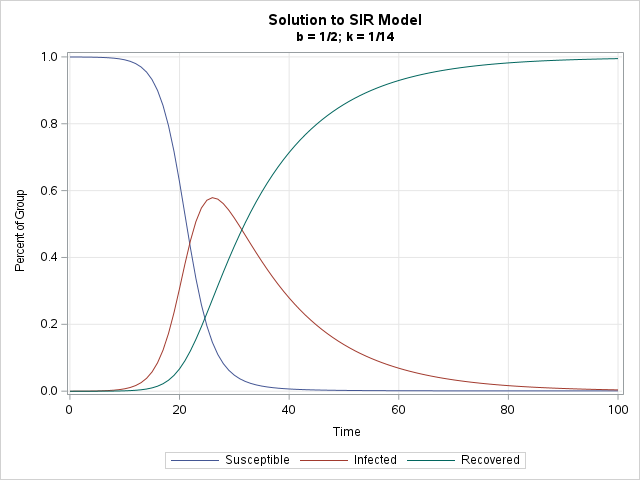
For the parameters (b, k) = (0.5, 0.07), the infected population rapidly increases until Day 25 when almost 60% of the population is infected. By this time, the population of susceptible people is only about 10% of the population. For these parameters, nearly everyone in the population becomes infected by Day 60. The highly infectious (but not lethal) epidemic is essentially over by Day 80 when almost everyone has been infected, recovered, and is now immune.

Example: An SIR model for a change in behavior

One of the advantages of mathematical models is that you can simulate "what if" scenarios. For example, what if everyone in the population changes their behavior on Day 20 to reduce the transmission rate? This might include the adoption of non-pharmaceutical interventions such as mask-wearing, social distancing, and quarantining the infected. What if these behaviors change the effective rate of transmission from 0.5 (very high) to 0.1 (moderate)? You can modify the module that defines the ODE to reflect that parameter change at t=20. As mentioned earlier, the ODEQN subroutine can integrate piecewise-defined systems if you specify the time at which the system changes its behavior. The following call to the ODEQN subroutine uses the TDISCONT= option to tell the integrator that the system of ODEs changes at t=20.

%let TChange = 20;
start SIR(t, y) global(k);
   if t < &TChange then b = 0.5;   /* more spread */
   else                 b = 0.1;   /* less spread */
 
   S = y[1]; I = y[2]; R = y[3];
   dSdt = -b * S*I;
   dIdt =  b * S*I - k*I;
   dRdt =            k*I;
   return ( dSdt || dIdt || dRdt );
finish;
 
/* set parameters and initial conditions */
k = 1/14;     /* k param: transition rate from I to R */
IC = {0.9999  0.0001   0};   /* S=99.99% I=0.01%  R=0 */
t = T(0:100);  /* compute spread for each day up to 100 days */
call odeqn(soln, "SIR", IC, t) TDISCON=&TChange;

If you plot the new solutions, you obtain the following graph:

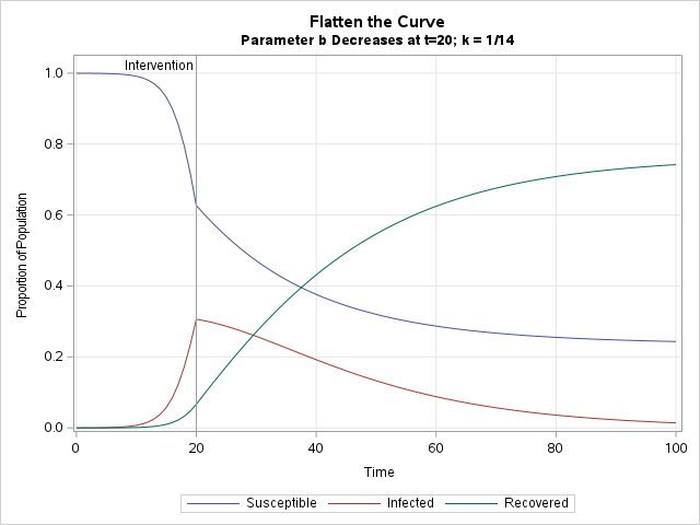
In the new scenario, the increase in the infected population is reversed by the intervention on Day 20. From there, the proportion of infected persons decreases over time. Eventually, the disease dies out. By Day 100, 75% of the population was infected and recovered, leaving 25% that are still susceptible to a future outbreak.

Summary

Although moving to SAS Viya offers many advantages for SAS customers who use Big Data and want to leverage parallel processing, Viya also provides new features for traditional SAS programmers. One example is the new ODEQN subroutine in SAS IML, which solves ODEs that are initial value problems by using state-of-the-art numerical algorithms. In addition to computational improvements in accuracy and speed, the ODEQN subroutine has a simple syntax and makes many decisions automatically, which makes the routine easier for non-experts to use.