Differential equations arise in the modeling of many physical processes, including mechanical and chemical systems. You can solve systems of first-order ordinary differential equations (ODEs) by using the ODE subroutine in the SAS/IML language, which solves initial value problems. This article uses the equations of motion for the classic simple harmonic oscillator to illustrate how to solve differential equations in SAS.
This article assumes that the parameters for the differential equations are known. If you need to estimate the parameters from data, see the paper by Erdman and Morelock (1996) and the examples in the documentation for the MODEL procedure in SAS/ETS software.
The simple harmonic oscillator: a linear system
A simple mechanical system is a spring with a mass at the end. If the spring obeys Hooke's Law and friction is ignored, Newton's Second Law dictates that the acceleration on the mass is proportional to the displacement of the mass from equilibrium. This leads to the second order differential equation x''(t) = -c x(t), which is the familiar differential equation for simple harmonic motion. (The prime indicates a derivative with respect to time.)Any higher-order differential equation can be rewritten as a system first-order of differential equations. The following SAS/IML module defines the first-order system for the standardized simple harmonic oscillator:
proc iml; /* Equations of motion for simple harmonic oscillator. This function returns the vector field evaluated at time t and location z. */ start SHO(t, z); dxdt = z[2]; /* dx/dt = v */ dvdt = -z[1]; /* dv/dt = -x */ return( dxdt // dvdt ); /* return column vector */ finish; |
Notice that because this differential equation is linear, you could also use matrix multiplication to define the module by using a single statement:
return( {0 1, -1 0}*z ); /* alternative approach */ |
The ODE subroutine solves differential equations. In addition to specifying the function that evaluates the vector field, you have to specify three parameters to the ODE subroutine:
- Initial conditions. For this example, I will use x0={2,0}, which corresponds to a mass that is displaced two units and released with no initial velocity. The initial condition should be specified as a column vector.
- A time interval that specifies the length of integration, [0, T]
- A vector that specifies the minimum, maximum, and initial steps for the variable-step-size integrator that the ODE subroutine uses. For this example, I will use the parameters h = {1.e-6 1 1e-3}.
For this example, I want to obtain and graph the solution at evenly spaced points in time. I can use a trick to accomplish this. If I specify a single time interval [0, T], I will obtain the final solution (x(T), v(T)). However, I can obtain the solution at multiple time points by specifying an increasing sequence such as t = do(0.2, 10, 0.2). This forces the ODS routine to return the solution at each of the specified time points.
The following statements define the parameters and call the ODE subroutine to compute the solution at a sequence of time points up to T = 10:
x0 = {2, 0};           /* initial values */
t = do(0, 10, 0.2);  /* compute solution at these time pts */
h = {1.e-6 1 1e-3};    /* min, max, and initial step size */
call ode(soln, "SHO", x0, t, h); |
The solution is returned in the soln matrix, which has two rows. Each column of the soln matrix contains the (x(t), v(t)) values for a specified value of t > 0.
Graphing the solution
The following statements write the ODE solution to a SAS data set and call the SGPLOT procedure to graph the solution as a function of time:
traj = t` || (x0` // soln`);
create SHO from traj[c={"Time" "x" "v"}];  /* write to data set */
append from traj;
close SHO;
quit; |
title "Simple Harmonic Motion"; proc sgplot data=SHO; label x="Position" v="Velocity"; series x=Time y=x; series x=Time y=v / y2axis; run; |
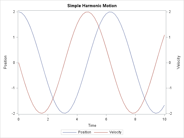
The position of the mass is described by a cosine function and the velocity (the derivative of position) is described by the negative sine function. This was expected because you can solve this simple linear system analytically.
There is a second way to graph the solution. The following statements display the solution as a parametric curve in the (x, v) plane.
title "One Trajectory for a Simple Harmonic Oscillator"; proc sgplot data=SHO aspect=1; /* the ASPECT= option is a SAS 9.4 feature */ series x=x y=v; xaxis grid label="Position"; yaxis grid label="Velocity"; run; |
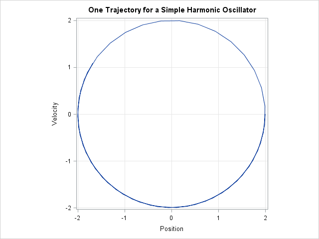
The parametric curve is a single trajectory of a "phase portrait," which can be used to analyze the qualitative dynamics of a system of differential equations. In my next blog post, I will show how to create a phase portrait in SAS.
