To a numerical analyst, numerical integration has two meanings. Numerical integration often means solving a definite integral such as $\int_{a}^b f(s) \, ds$. Numerical integration is also called quadrature because it computes areas. The other meaning applies to solving ordinary differential equations (ODEs). My article about new methods for solving ODEs in SAS uses the words "integrate" and "integrator" a lot. This article caused a colleague to wonder about the similarities and differences between integration as a method for solving a definite integral and integration as a method for solving an initial-value problem for an ODE. Specifically, he asked whether you could use an ODE solver to solve a definite integral?

It is an intriguing question. This article shows that, yes, you can use an ODE solver to compute some definite integrals. However, just as a builder should use the most appropriate tools to build a house, so should a programmer use the best tools to solve numerical problems. Just because you can solve an integral by using an ODE does not mean that you should discard the traditional tried-and-true methods of solving integrals.

The most famous differential equation in probability and statistics

However, there is a problem. By integrating both sides of the differential equation, you obtain $F(x) = \int_{-\infty}^x f(s) \, ds$. Because the lower limit of integration is -∞, you cannot solve the differential equation as an initial-value problem (IVP). An initial-value problem requires that you know the value of the function for some finite value of the lower limit.

However, you can get around this issue for some specific distributions. Some distributions have a lower limit of 0 instead of -∞. If the density at x=0 is finite, you can solve the ODE for those distributions.

You can also use an ODE to solve for the CDF of symmetric distributions. If f is a symmetric distribution, the point of symmetry is the median value of the distribution. So, if s₀ is the symmetric value, you can solve the ODE $F^\prime(x) = f(x)$ for any value x ≥ s₀ by using the initial condition $F(s_0) = 0.5$. Thus, you can use an IVP solve any integral of the form $\int_{s_0}^b f(s) \, ds$. By symmetry, you can solve any integral of the form $\int_a^{s_0} f(s) \, ds$. By combining these results, you can use an IVP to solve the integral on any finite-length interval [a, b].

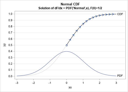
This symmetry idea is shown in the graph to the right for the case of the standard normal distribution. The normal distribution is symmetric about the median s₀=0. This means that the CDF passes through the point (0, 1/2). You can integrate the ODE to obtain the CDF curve for any positive value of x. The computations are shown in the next section.

Solve an integral to find the normal probability

I like to know the correct answer BEFORE I do any computation. The usual way to compute an integral in SAS is to use the QUAD subroutine in SAS/IML software. (QUAD is short for quadrature.) This subroutine is designed to compute one-dimensional integrals. To use the QUAD subroutine, you need to define the integrand and interval of integration. For example, the following statements define the integral for the normal PDF on the interval [0, 3]:

proc iml;
/* Use QUAD subroutine to integrate the standard normal PDF.
   Note: For this integrand, you can call the CDF function to compute the integral:
         CDF = cdf("Normal", 3) - 0.5; */
start NormalPDF(x);
   return pdf("Normal", x);   /* f(x) = 1/sqrt(2*pi) *exp(-x##2/2) */
finish;
 
/* find the area under pdf on [0, 3] */
call quad(Area, "NormalPDF", {0 3});
print Area;

The QUAD subroutine makes it simple to integrate any continuous function on a finite interval. In fact, the QUAD subroutine can also integrate over infinite intervals! And, if you specify the points of discontinuity, it can integrate functions that are not continuous at finitely many points.

Solve an ODE to find the normal probability

Just for fun, let's see if we can get the same answer by using the ODE subroutine to solve a differential equation. We want to compute the integral $F(a) = \int_0^a \phi(s) \, ds$, where φ is the standard normal PDF. The equivalent formulation as a differential equation is $F^{\prime}(x) = \phi(x)$, where F(0)=0.5. For this example, we want to solution at x=3.

The module that evaluates the right-hand side of the ODE must take two arguments. The first argument is the independent variable, which is x. The second argument is the state of the system, which is not used for this problem. You also need to specify the initial condition, which is F(0)=0.5. Lastly, you also need to specify the limits of integration which is [0, 3]. The following statements use the ODE subroutine in SAS/IML software to solve the IVP defined by F`(x)=PDF("Normal",x) and F(0)=0.5:

/* ODE is A` = 1/sqrt(2*pi) *exp(-x##2/2) 
   A(0) = 0.5  */
start NormalPDF_ODE(s, y);
   return pdf("Normal", s);
finish;
 
c = 0.5;                     /* initial value at x=0 */
x = {0 3};                  /* integrate from x=0 to x=3 */
h={1.e-7, 1, 1e-4};          /* (min, max, initial) step size for integrator */
call ode(result, "NormalPDF_ODE", c, x, h) eps=1e-7;
A = result - c;
print A;

Success! The ODE gives a similar numerical result for the integral of the PDF, which is the CDF at x=3.

Integrating an ODE is a poor way to compute an integral

Although it is possible to use an ODE to solve some integrals on a finite domain, this result is more of a curiosity than a practical technique. A better choice is to use a routine designed for numerical integration, such as the QUAD subroutine. The QUAD subroutine can integrate on any domain, including infinite domains. For example, the following statements integrate the normal PDF on [-3, 3] and (-∞, 3), respectively.

call quad(Area2, "NormalPDF", {-3 3});  /* area on [-3, 3] */
call quad(Area3, "NormalPDF", {0 .P});  /* area on [0, infinity) */
print Area2 Area3;

In addition, the QUAD subroutine can be used to compute double integrals by using iterated integrals. As far as I know, you cannot use an ODE to compute a double integral.

Whereas the ODE subroutine requires knowing an initial value on the curve, the QUAD routine does not. The ODE subroutine also requires separate calls to integrate forward and backward from the initial condition, whereas the QUAD routine does not.

Summary

The phrase "numerical integration" has two meanings in numerical analysis. The usual meaning is "quadrature," which means to evaluate a definite integral. However, it is also used to describe the numerical solution of an ODE. In certain cases, you can use an ODE to solve a definite integral on a bounded domain. However, the ODE requires special additional information such as knowing an "initial condition." So, yes, you can (sometimes) solve integrals by using a differential equation, but the process is more complicated than if you use a standard method for solving integrals.