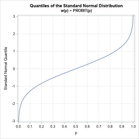
The graph to the right is the quantile function for the standard normal distribution, which is sometimes called the probit function. Given any probability, p, the quantile function gives the value, x, such that the area under the normal density curve to the left of x is exactly p. This function is the inverse of the normal cumulative distribution function (CDF).
Did you know that this curve is also the solution of a differential equation? You can write a nonlinear second-order differential equation whose solution is exactly the probit function! This means that you can compute quantiles by solving a differential equation.
This article derives the differential equation and solves it by using the built-in ODE subroutine in SAS/IML software.
A differential equation for quantiles
Let w(p) = PROBIT(p) be the standard normal quantile function.
The w function satisfies the following differential equation:
\(\frac{d^2w}{dp^2} = w \left( \frac{dw}{dp}\right)^2\)
The derivation of this formula is shown in the appendix.
A differential equation looks scary, but it merely reveals a relationship between the derivatives of a function at every point in the domain. For example: at the point p=1/2, the value of the probit function is w(1/2) = 0, and the slope of the function is w'(1/2) = sqrt(2 π). From those two values, the differential equation tells you that the second derivative at p=0 is exactly 0*2π = 0.
The appendix shows how to use calculus to prove the relationship. You can also use the NLPFDD subroutine in SAS/IML to compute finite-difference derivatives at an arbitrary value of p. The derivatives satisfy the differential equation to within the accuracy of the computation.
Use the differential equation to compute quantiles
An interesting application of the ordinary differential equation (ODE) is that you can use it to compute quantiles. At the point, p=1/2, the probit function has the value w(1/2) = 0, and the slope of the function is w'(1/2) = sqrt(2 π). Therefore, the probit function is the particular solution to the previous ODE for those initial conditions. Consequently, you can obtain the quantiles by solving an initial value problem (IVP).
I previously showed how to use the ODE subroutine in SAS/IML to solve initial value problems. For many IVPs, the independent variable represents time, and the solution represents the evolution of the state of the system, given an initial state. For this IVP, the independent variable represents probability. By knowing the quantile of the standard normal distribution at one location (p=1/2), you can find any larger quantile by integrating forward, or any smaller quantile by integrating backward.
The ODE subroutine solves systems of first-order differential equations, so you must convert the second-order equation into a system that contain two first-order equations. Let v = dw/dp = w`. Then the differential equation can be written as the following first order system:
w` = v v` = w * v**2 |
The following SAS/IML statement use the differential equation to find the quantiles of the standard normal distribution for p={0.5, 0.68, 0.75, 0.9, 0.95, 0.99}:
proc iml;
/* Solve first-order system of ODES with IC
   w(1/2) = 0
   v(1/2) = sqrt(2*pi)
*/
start NormQntl(t,y);
   w = y[1]; v = y[2];
   F = v  // w*v**2;
   return(F);
finish;

/* initial conditions at p=1/2 */
pi = constant('pi');
c = 0 || sqrt(2*pi);

/* integrate forward in time to find these quantiles */
p = {0.5, 0.68, 0.75, 0.9, 0.95, 0.99};

/* ODE call requires a column vector for the IC, and a row vec for indep variable */
c = colvec(c);               /* IC */
t = rowvec(p);               /* indep variable */
h={1.e-7, 1, 1e-4};          /* (min, max, initial) step size for integrator */
call ode(result, "NormQntl", c, t, h) eps=1e-6;
Traj  = (c` // result`);     /* solutions in rows. Transpose to columns */
qODE = Traj[,1];             /* first column is quantile; second col is deriv */

/* compare with the correct answers */
Correct = quantile("Normal", p);
Diff = Correct - qODE;       /* difference between ODE solution and QUANTILE */
print p Correct qODE Diff; |
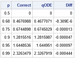
The output shows the solution to the system of ODEs at the specified values of p. The solution is very close to the more exact quantiles as computed by the QUANTILE function. This is fairly impressive if you think about it. The ODE subroutine has no idea that it is solving for normal quantiles. The subroutine merely uses a general-purpose ODE solver to generate a solution at the specified values of p. In contrast, the QUANTILE routine is a special-purpose routine that is engineered to produce the best-possible approximations of the normal quantiles.
To get quantiles for p < 0.5, you can use the symmetry of the normal distribution. The quantiles satisfy the relation w(1-p) = -w(p).
Summary
A differential equation reveals the relationship between a function and its derivatives. It turns out that there is an ordinary differential equation that is satisfied by the quantile function of any smooth probability distribution. This article shows the ODE for the standard normal distribution. You can solve the ODE in SAS to compute quantiles if you also know the value of the quantile function and its derivative at some point, such as a median at p=1/2.
Appendix: Derive the quantile ODE
For the mathematically inclined, this section derives a differential equation for any smooth probability distribution. The equations are given in a Wikipedia article, but the article does not include a derivation.
Let X be a random variable that has a smooth CDF, F. The density function, f, is the first derivative of F. By definition, the quantile function, w, is the inverse of the CDF function. That means that for any probability, p, the CDF and quantile function satisfy the equation \(F(w(p)) = p\).
Take the deivative of both sides with respect to p and apply the chain rule:
\(F^\prime(w(p)) \frac{dw}{dp} = 1\)
Substitute f for the derivative and solve for dw/dp:
\(\frac{dw}{dp} = \frac{1}{f(w(p))}\)
Again, take the derivative of both sides:
\(\frac{d^2w}{dp^2} = \frac{-1}{f(w(p))^2} \frac{df}{dp} \frac{dw}{dp}\).
You can use the relationship dw/dp = 1/f to obtain
\(\frac{d^2w}{dp^2} = \frac{-f(w)^\prime}{f(w)} \left( \frac{dw}{dp} \right)^2\).
In this derivation, I have not used any special properties of the distribution. Therefore, it is satisfied by any probability distribution that is sufficiently smooth and for any values of p for which the equation is well-defined.
The ODE simplifies for some probability density functions. For example, the standard normal density is
\(f(w) = \frac{1}{\sqrt{2\pi}} \exp(-w^2/2 )\) and thus
\(f^\prime(w) = \frac{1}{\sqrt{2\pi}} \exp(-w^2/2 )(-w) = -f(w) w\).
Consequently, for the standard normal distribution, the ODE simplifies to
\(\frac{d^2w}{dp^2} = w \left( \frac{dw}{dp}\right)^2\).

2 Comments
I love all your non linear and numerical analysis posts. Can we do something like this with the hash object?
Thanks! There are many ways to estimate quantiles from data. Is that what you mean? I do not know how to solve a differential equation by using the hash object.