Sometimes it is useful to know the extreme values in data. You might need to know the Top 5 or the Top 10 smallest data values. Or, the Top 5 or Top 10 largest data values. There are many ways to do this in SAS, but this article shows examples that use four different methods to find the top k or bottom k data values:

1. Use the NEXTROBS= option in PROC UNIVARIATE to output the N EXTReme OBServations. This is by far the easiest method.
2. Sort the data in ascending or descending order. Display the top k rows.
3. Transpose the data to make a wide data set. Use the SMALLEST and LARGEST functions in the SAS DATA step to obtain the k largest or smallest data values.
4. If the data contain ties values, you might want to find the largest or smallest unique values. For that task, you can use the NEXTRVAL= option in PROC UNIVARIATE, or you can use PROC RANK.

This article discusses how to find the most extreme data values for a continuous (interval) variable. Each method has different ways to handle missing values and tied values.

A related question is finding the most frequently observed categories for a categorical variable. If you are interested in making a Top 10 list or bar chart of a categorical variable, see the article, "An easy way to make a "Top 10" table and bar chart in SAS."

Example data

The following SAS DATA step defines a variable that has 100 observations. Each value is in the interval [0, 4]. and some of the values are repeated.

/* 100 values. One missing value. Nonmissing values in [0, 4].
   Tied values include 0.02 (two times) and 0.03 (three times)
*/
data Have;
input x @@;
datalines;
0.54 3.33 2.55 0.95 1.11 1.02 1.09 1.78 2.87 2.53
   . 1.49 0.74 0.02 0.29 0.17 1.08 0.21 4.00 0.83
0.09 2.25 2.56 1.93 0.34 0.31 0.08 0.29 0.65 0.08
0.78 0.08 0.83 0.01 0.46 1.22 0.53 0.07 0.08 0.46
0.59 0.04 0.26 0.68 0.10 1.91 0.31 0.24 0.05 1.04
0.24 0.10 0.09 0.03 0.30 2.98 0.33 0.18 0.22 2.50
2.41 2.66 0.22 0.60 2.32 1.17 1.14 0.05 0.56 0.42
2.87 0.03 0.40 0.44 0.23 1.64 0.31 1.00 1.96 0.08
0.10 0.06 1.24 0.03 0.63 1.14 0.07 0.06 0.13 1.83
1.14 0.18 0.13 0.75 0.69 1.62 2.27 1.50 0.02 1.04 
;

There is a missing value for the X variable. The value 0.02 is repeated twice. The value 0.03 is repeated three times. The five smallest nonmissing values are {0.01, 0.02, 0.02, 0.03, 0.03, 0.03}.

Use PROC UNIVARIATE

The simplest way to see the k largest and smallest observations is to use the NEXTROBS= option on the PROC UNIVARIATE statement. You can specify the number of extreme observations that you wish to see. For example, the following statements ask for k=5 extreme observations:

%let nTop = 5;  /* display the Top 5 largest and smallest values */
 
proc univariate data=Have NExtrObs=&nTop;
   var x;
   ods select ExtremeObs;
run;

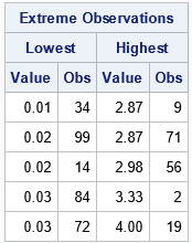
The table shows that the Top 5 smallest values are 0.01, 0.02, 0.02, 0.03, and 0.03. It provides the observations numbers (rows) for each value. Similarly, the table shows that the Top 5 largest values are 2.87, 2.87, 2.98, 3.33, and 4.00. The output also shows that tied values are handled arbitrarily. Although the value 0.03 appears three times in the data, the table does not reveal that information.

However, you can also use PROC UNIVARIATE to find the k smallest and largest UNIQUE values. To do this, specify the NEXTRVAL= option, as follows:

proc univariate data=Have NExtrObs=&nTop NExtrVal=&nTop ;
   var x;
   ods select ExtremeObs ExtremeValues;
run;

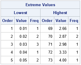
The second table shows that the value 0.02 appears twice in the data. The value 0.03 appears three times, and so on. This table is useful when you have many tied values in the data.

PROC UNIVARIATE is the simplest and most flexible way to display extreme values. By adding additional variables to the VAR statement, it is easy to report this information for several continuous variables.

Although PROC UNIVARIATE is the best way, I often see other suggestions made on discussion forums. For completeness, the rest of the article discusses alternative ways to report the smallest and largest observations in univariate data.

The sorting method

The sorting method is conceptually easy. If you sort the data in increasing order, the first few observations are the smallest. If you sort the data in decreasing order, the first few observations are the largest. You can use PROC SORT and PROC PRINT to reveal the largest and smallest values for the X variable:

%let nTop = 5;  /* display the Top 5 largest and smallest values */
 
proc sort data=Have out=SortInc;  by x;  run;
proc sort data=Have out=SortDec;  by descending x;  run;
 
proc print data=SortInc(obs=&nTop keep=x rename=(x=Smallest)); run;
proc print data=SortDec(obs=&nTop keep=x rename=(x=Largest)); run;

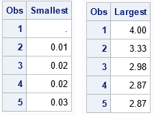
The tables show the smallest and largest values as computed by sorting the data. By convention, a missing value in SAS is smaller than any double-precision floating-point value. Thus, the list of smallest values includes the missing value. The output also shows that tied values are handled arbitrarily, as for the NEXTROBS= option in PROC UNIVARIATE.

Notice that PROC UNIVARIATE automatically excluded missing observations. If you use the sorting method and do not want the missing value to appear, you can use a WHERE clause to filter it out:

proc sort data=Have out=SortInc;
   where not missing(x);         /* exclude missing values from the smallest values */
   by x;  
run;

The sorting method is conceptually easy to implement. A disadvantage is that it creates two copies of the data: one for the ascending case and another for the descending case. After you create the data sets, it is easy to ask for the Top 5, Top 10, or Top 20 values without requiring additional computation. However, it is not well suited if you want to report extreme values for multiple variables.

The SMALLEST and LARGEST functions

The SAS DATA step supports the SMALLEST and LARGEST functions, which returns the kth smallest and largest values in an array, respectively. That is, the SMALLEST and LARGEST functions are designed to work on rows of data, whereas the sorting data works on columns.

You can transpose the values, put them in a temporary array, and use the SMALLEST and LARGEST functions to find the extreme values in the data. To use this technique, you first need to know how many values exist so that you can allocate an array of the correct size. The following DATA step uses a standard technique to discover the number of rows in a data set. Then the X variable is read into a temporary array. After the data are read, the SMALLEST and LARGEST functions are called multiple times to obtain the results:

/* discover the number of rows in a data set */
data _NULL_;
if 0 then 
   set Have NOBS=nRows;
call symputx('nRows', nRows);  /* put number of rows into macro variable */
stop;
run;
%put &=nRows;
 
/* DATA step supports the SMALLEST and LARGEST functions for rows */
data SmallLarge;
array v[&nRows] _temporary_;
set Have nobs=nObs end=eof;
v[_N_] = x;
if eof then do;
   do k = 1 to &nTop;
      Smallest = smallest(k, of v[*]);
      Largest = largest(k, of v[*]);
      output;
   end;
end;
keep k Smallest Largest;
run;
 
proc print data=SmallLarge;
run;

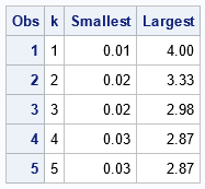
The SMALLEST and LARGEST functions are great for finding extreme values in a row of data. However, for data in a column, this example shows that this DATA step method is more complicated to implement than the procedure-based methods. Unlike the sorting method, it does not create copies of the data set on a disk. However, it does keep a copy in RAM. A disadvantage to this method is that each call to the SMALLEST and LARGEST functions traverses the array. Thus, this method can be inefficient. If you use it to generate a list of the 50 smallest values, the array is traversed 50 times.

The ranking method

You can use PROC RANK to assign a rank to each value. PROC RANK has several methods for ranking tied values. For this application, use the TIES=DENSE option. The following statements show how to display the smallest values for a variable. If you use the DESCENDING option on the PROC RANK statement, you obtain the largest values:

proc rank data=Have out=RankOutInc ties=DENSE /* Optional: DESCENDING */;
   var x;
   ranks Rank;
run;
 
proc print data=RankOutInc;
   where Rank <= &nTop & not missing(Rank);
run;

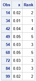
Because tied values are assigned the same ranks, this method is similar to using the NEXTRVAL= option in PROC UNIVARIATE. You can see, however, that PROC RANK does not reorder the data values. Although the table shows the five smallest values in the data, they are not displayed in a sorted order.

Summary

In summary, there are several ways to use SAS to find the Top 5 (or Top 10) smallest and largest values in data. I recommend using the NEXTROBS= option on the PROC UNIVARIATE statement. Not only is it easy to use, but you can display the smallest/largest values for multiple variables. For comparison, this article presents several alternative methods including sorting, using the SMALLEST and LARGEST functions, and using PROC RANK. These methods are less convenient than PROC UNIVARIATE.