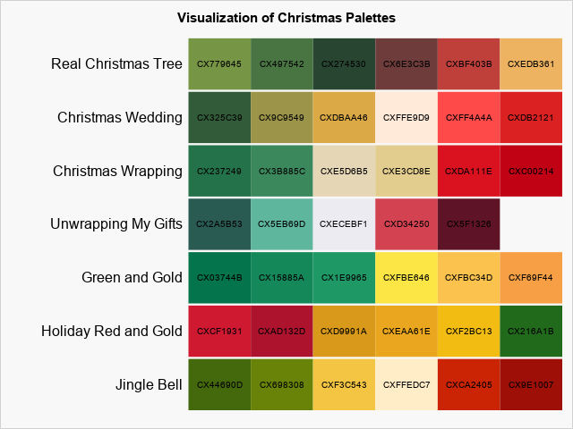
In a previous article, I visualized seven Christmas-themed palettes of colors, as shown to the right. You can see that the palettes include many red, green, and golden colors. Clearly, the colors in the Christmas palettes are not a random sample from the space of RGB colors. Rather, they represent a specific subset of Christmas colors. I thought it would be fun to use principal component analysis to compute and visualize the linear subspace that best captures the set of Christmas colors!

Convert hexadecimal colors to RGB

Each color can be represented as an ordered triplet of unsigned integers in RGB space. The colors in SAS are 8-bit colors, which means that each coordinate in RGB space has a value between 0 and 255. The following DATA step reads the colors in the Christmas palettes and uses the HEX2. informat to convert the hexadecimal values to their equivalent RGB values. As explained in the previous article, the DATA step also creates an ID value for each color and creates a macro variable (AllColors) that contains the list of all colors.

/* read Christmas palettes. Convert hex to RGB */
data RGB;
length Name $30 color $8;
length palette $450; /* must be big enough to hold all colors */
retain ID 1 palette;
input Name 1-22 n @;
do col = 1 to n;
   input color @;
   R = inputn(substr(color, 3, 2), "HEX2."); /* get RGB colors from hex */
   G = inputn(substr(color, 5, 2), "HEX2.");
   B = inputn(substr(color, 7, 2), "HEX2.");
   palette = catx(' ', palette, color);
   output;
   ID + 1;                             /* assign a unique ID to each color */
end;
call symput('AllColors', palette);   /* concatenate colors; store in macro */
drop n col palette;
/* Palette Name      |n| color1 | color2 | color2 | color4 | ... */
datalines;
Jingle Bell           6 CX44690D CX698308 CXF3C543 CXFFEDC7 CXCA2405 CX9E1007
Holiday Red and Gold  6 CXCF1931 CXAD132D CXD9991A CXEAA61E CXF2BC13 CX216A1B
Green and Gold        6 CX03744B CX15885A CX1E9965 CXFBE646 CXFBC34D CXF69F44
Unwrapping My Gifts   5 CX2A5B53 CX5EB69D CXECEBF1 CXD34250 CX5F1326
Christmas Wrapping    6 CX237249 CX3B885C CXE5D6B5 CXE3CD8E CXDA111E CXC00214
Christmas Wedding     6 CX325C39 CX9C9549 CXDBAA46 CXFFE9D9 CXFF4A4A CXDB2121
Real Christmas Tree   6 CX779645 CX497542 CX274530 CX6E3C3B CXBF403B CXEDB361
;

The result of this DATA step is a data set that contains 41 rows. The R, G, and B variables contain the red, green, and blue components, respectively, which are in the range 0 to 255. Thus, the data contains 41 triplets of RGB values.

Let's use PROC PRINCOMP in SAS to run a principal component analysis of these 41 observations:

proc princomp data=RGB N=2 out=PCOut plots(only)=(Score Pattern);
   var R G B;
   ID color;
run;

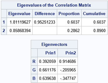
Recall that each principal component is a linear combination of the original variables (R, G, and B). The table shows that the first principal component (PC) is the linear combination
PC₁ = 0.39*R + 0.66*G + 0.64*B
The first PC is a weighted sum of the amount of color across all three variables. More weight is given to the green and blue components than to the red component. Along the axis of the first PC, black is on the extreme left since black has the RGB value (0, 0, 0). Similarly, white is on the extreme right since white has the RGB value (255, 255, 255).

The second principal component is the linear combination
PC₂ = 0.91*R - 0.21*G - 0.35*B
The second PC is a contrast between the red coordinate and the green and blue coordinates. Along the axis of the second PC, colors that have a lot of green and blue (such as cyan, which is (0, 255, 255)) have extreme negative values whereas colors that are mostly red have extreme positive values.

An additional table (not shown) indicates that 89% of the variation in the data is explained by using the first two principal components. You could add a third principal component if you want to have a way to separate the green and blue colors.

The PRINCOMP procedure creates a graph that projects each RGB value onto the principal component axes. Because I put the COLOR variable on the ID statement, each marker is labeled by using its hexadecimal value:

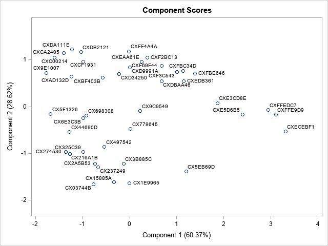
This graph shows how the colors in the Christmas palettes are distributed in the space of the first two PCs. However, wouldn't it be cool if the markers in this plot were the colors that the markers represent? The next section adds color to the scatter plot by using PROC SGPLOT.

Adding color to the score plot

The previous call to PROC PRINCOMP includes the OUT= option, which writes the principal component scores to a SAS data set. The names of the scores are PRIN1 and PRIN2. If you use the PRIN1 and PRIN2 variables to create a scatter plot, you can re-create the score plot from PROC PRINCOMP. However, I am going to add a twist. As shown in my previous post, I will use the GROUP= option to specify that the marker colors be assigned according to the value of the ID variables, which are the integers 1, 2, ..., 41. I will use the STYLEATTRS statement and the DATACONTRASTCOLORS= option to specify that the colors that should be used for each group. The result is a scatter plot in which each marker is colored according to a specified list of colors.

title "Principal Component Scores for Christmas Colors";
proc sgplot data=PCOut noautolegend aspect=1;
   label Prin1="Component 1 (60.37%)" Prin2="Component 2 (28.62%)";
   styleattrs datacontrastcolors=(&AllColors);
   scatter x=Prin1 y=Prin2 / markerattrs=(symbol=CircleFilled size=16) group=ID;
   refline 0 / axis=x;
   refline 0 / axis=y;
run;

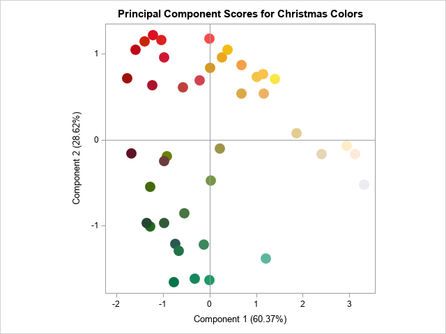
The graph shows the distribution of the colors, using the colors themselves as a visual cue. The graph shows that the first PC differentiates between dark colors (on the left) and light colors (on the right). The second PC differentiates between blue-green colors (on the bottom) and red colors (on the top).

Summary

I almost titled this article, "A Statistician Looks at Christmas Colors." I started with a set of Christmas-themed palettes with 41 colors that were primarily red, green, and gold. By performing a principal component analysis, you can project the RGB coordinates of these colors onto the plane that captures most of the variation in the data. If you color the markers in this projection, you obtain a scatter plot that shows green colors in one region, red colors in another region, and gold and silver colors in yet another.

The graph shows the various Christmas colors in one image. To me, the image seems more coherent and organized than the original strips of colors. I like that similar colors are grouped together, and that the three groups of colors (red, green, and blue) are visibly distinct.

If you want to experiment with other color palettes, you can download the SAS program that computes all graphs in this article.