Examples of using the Hoeffding D statistic

A previous article discusses the definition of the Hoeffding D statistic and how to compute it in SAS. The letter D stands for "dependence." Unlike the Pearson correlation, which measures linear relationships, the Hoeffding D statistic tests whether two random variables are independent. Dependent variables have a Hoeffding D statistic that is greater than 0. In this way, the Hoeffding D statistic is similar to the distance correlation, which is another statistic that can assess dependence versus independence.

This article shows a series of examples where Hoeffding's D is compared with the Pearson correlation. You can use these examples to build intuition about how the D statistic performs on real and simulated data.

Hoeffding's D and duplicate values

As a reminder, Hoeffding's D statistic is affected by duplicate values in the data. If a vector has duplicate values, the Hoeffding association of the vector with itself will be less than 1. A vector that has many duplicate values (few distinct values) has an association with itself that might be much less than 1.

For many examples, the Hoeffding D association between two variables is between 0 and 1. However, occasionally you might see a negative value for Hoeffding's D, especially if there are many duplicate values in the data.

Pearson correlation versus Hoeffding's D on real data

Let's compare the Pearson correlation and the Hoeffding D statistic on some real data. The following call to PROC SGSCATTER creates bivariate scatter plots for five variables in the Sashelp.Cars data set:

%let VarList = MSRP Invoice EngineSize Horsepower MPG_City MPG_Highway;
proc sgscatter data=sashelp.cars;
   matrix &VarList;
run;

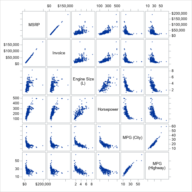
The graph shows relationships between pairs of variables. Some pairs (MSRP and Invoice) are highly linearly related. Other pairs (MPG_City versus other variables) appear to be related in a nonlinear manner. Some pairs are positively correlated whereas others are negatively correlated.

Let's use PROC CORR in SAS to compare the matrix of Pearson correlations and the matrix of Hoeffding's D statistics for these pairs of variables. The NOMISS option excludes any observations that have a missing value in any of the specified variables:

proc corr data=Sashelp.cars PEARSON HOEFFDING noprob nomiss nosimple;
   label EngineSize= MPG_City= MPG_Highway=; /* suppress labels */
   var &VarList;
run;

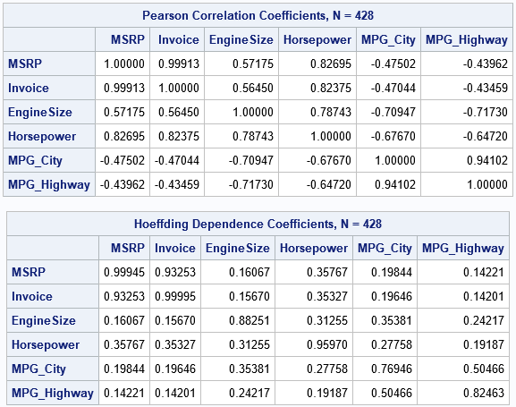
There are a few noteworthy differences between the tables:

Diagonal elements: For these variables, there are 428 complete cases. The Invoice variable has 425 unique values (only three duplicates) whereas the MPG_City and MPG_Highway variables have only 28 and 33 unique values, respectively. Accordingly, the diagonal elements are closest to 1 for the variables (such as MSRP and Invoice) that have few duplicate values and are smaller for variables that have many duplicate values.
Negative correlations: A nice feature of the Pearson correlation is that it reveals positive and negative relationships. Notice the negative correlations between MPG_City and other variables. In contrast, the Hoeffding association assesses dependence/independence. The association between MPG_City and the other variables is small, but the table of Hoeffding statistics does not give information about the direction of the association.
Magnitudes: The off-diagonal Hoeffding D statistics are mostly small values between 0.15 and 0.35. In contrast, the same cells for the Pearson correlation are between -0.71 and 0.83. As shown in a subsequent section, the Hoeffding statistic has a narrower range than the Pearson correlation does.

Association of exact relationships

A classic example in probability theory shows that correlation and dependence are different concepts. If X is a random variable and Y=X², then X and Y are not independent, even though their Pearson correlation is 0. The following example shows that the Hoeffding statistic is nonzero, which indicates dependence between X and Y:

data Example;
do x = -1 to 1 by 0.05;          /* X is in [-1, 1] */
   yLinear = 3*x + 2;            /* Y1 = 3*X + 2    */
   yQuad   = x**2 + 1;           /* Y2 = X**2 + 1   */
   output;
end;
run;
 
proc corr data=Example PEARSON HOEFFDING nosimple noprob;
   var x YLinear yQuad;
run;

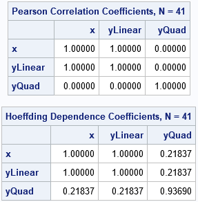
Both statistics (Pearson correlation and Hoeffding's D) have the value 1 for the linear dependence between X and Y_Linear. The Pearson correlation between X and Y_Quad is 0, whereas the Hoeffding D statistic is nonzero. This agrees with theory: the two random variables are dependent, but their Pearson correlation is 0.

Statistics for correlated bivariate normal data

A previous article about distance correlation shows how to simulate data from a bivariate normal distribution with a specified correlation. Let's repeat that numerical experiment, but this time compare the Pearson correlation and the Hoeffding D statistic. To eliminate some of the random variation in the statistics, let's repeat the experiment 10 times and plot the Monte Carlo average of each experiment. That is, the following SAS/IML program simulates bivariate normal data for several choices of the Pearson correlation. For each simulated data set, the program computes both the Pearson correlation and Hoeffding's D statistic. This is repeated 10 times, and the average of the statistics is plotted:

proc iml;
call randseed(54321);
 
/* helper functions */
start PearsonCorr(x,y);
   return( corr(x||y)[1,2] );
finish;
start HoeffCorr(x,y);
   return( corr(x||y, "Hoeffding")[1,2] );
finish;
 
/* grid of correlations */
rho = {-0.99 -0.975 -0.95} || do(-0.9, 0.9, 0.1) || {0.95 0.975 0.99};  
N = 500;                   /* sample size */
mu = {0 0};  Sigma = I(2); /* parameters for bivariate normal distrib */
PCor = j(1, ncol(rho), .); /* allocate vectors for results */
HoeffD = j(1, ncol(rho), .);
 
/* generate BivariateNormal(rho) data */
numSamples = 10;           /* how many random samples in each study? */
do i = 1 to ncol(rho);     /* for each rho, simulate bivariate normal data */
   Sigma[1,2] = rho[i]; Sigma[2,1] = rho[i]; /* population covariance */
   meanP=0; meanHoeff=0;   /* Monte Carlo average in the study */
   do k = 1 to numSamples;
      Z = RandNormal(N, mu, Sigma);        /* simulate bivariate normal sample */
      meanP = meanP + PearsonCorr(Z[,1], Z[,2]);        /* Pearson correlation */
      meanHoeff = meanHoeff + HoeffCorr(Z[,1], Z[,2]);  /* Hoeffding D */
   end;
   PCor[i] = MeanP /numSamples;             /* MC mean of Pearson correlation */
   HoeffD[i] = meanHoeff / numSamples;      /* MC mean of Hoeffding D */
end;
 
create MVNorm var {"rho" "PCor" "HoeffD"}; 
append; close;
QUIT;
 
title "Average Correlations/Associations of Bivariate Normal Data";
title2 "N = 500";
proc sgplot data=MVNorm;
   label rho="Pearson Correlation of Population"
         PCor="Pearson Correlation"
         HoeffD="Hoeffding's D";
   series x=rho y=PCor / markers name="P";
   series x=rho y=HoeffD / markers name="D";
   lineparm x=0 y=0 slope=1;
   yaxis grid label="Association or Correlation";
   xaxis grid;
   keylegend "P" "D";
run;

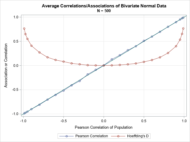
For these bivariate normal samples (of size 500), the Monte Carlo means for the Pearson correlations are very close to the diagonal line, which represented the expected value of the correlation. For the same data, the Hoeffding D statistics are different. For correlations in [-0.3, 0.3], the mean of the D statistic is positive and is very close to 0. Nevertheless, the p-values for the Hoeffding test of independence account for the shape of the curve. For bivariate normal data that has a small correlation (say, 0.1), the Pearson test for zero correlation and the Hoeffding test for independence often both accept or both reject their null hypotheses.

Summary

Hoeffding's D statistic provides a test for independence, which is different than a test for correlation. In SAS, you can compute the Hoeffding D statistic by using the HOEFFDING option on the PROC CORR statement. You can also compute it in SAS/IML by using the CORR function. Hoeffding's D statistic can detect nonlinear dependencies between variables. It does not, however, indicate the direction of dependence.

I doubt Hoeffding's D statistic will ever be as popular as Pearson's correlation, but you can use it to detect nonlinear dependencies between pairs of variables.

Blogs