Correlation is a statistic that measures how closely two variables are related to each other. The most popular definition of correlation is the Pearson product-moment correlation, which is a measurement of the linear relationship between two variables. Many textbooks stress the linear nature of the Pearson correlation and emphasize that a zero value for the Pearson correlation does not imply that the variables are independent. A classic example is to define X to be a random variable on [-1, 1] and define Y=X². X and Y are clearly not independent, yet you can show that the Pearson correlation between X and Y is 0.

In 2007, G. Szekely, M. Rizzo, and N. Bakirov published a paper in the The Annals of Statistics called "Measuring and Testing Dependence by Correlation of Distances." This paper defines a distance-based correlation that can detect nonlinear relationships between variables. This blog post describes the distance correlation and implements it in SAS.

An overview of distance correlation

It is impossible to adequately summarize a 27-page paper from the Annals in a few paragraphs, but I'll try. The Szekely-Rizzo-Bakirov paper defines the distance covariance between two random variables. It shows how to estimate the distance correlation from data samples. A practical implication is that you can estimate the distance correlation by computing two matrices: the matrix of pairwise distances between observations in a sample from X and the analogous distance matrix for observations from Y. If the elements in these matrices co-vary together, we say that X and Y have a large distance correlation. If they do not, they have a small distance correlation.

For motivation, recall that the Pearson covariance between X and Y (which is usually defined as the inner product of two centered vectors) can be written in terms of the raw observations:

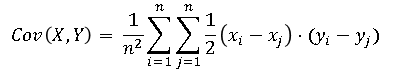
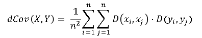
The terms (x_i – x_j) and (y_i – y_j) can be thought of as the one-dimensional signed distances between the i_th and j_th observations. Szekely et al. replace those terms with centered Euclidean distances D(x_i, x_j) and define the distance covarariance as follows:

The distance covariance between random vectors X and Y has the following properties:

• X and Y are independent if and only if dCov(X,Y) = 0.
• You can define the distance variance dVar(X) = dCov(X,X) and the distance correlation as dCor(X,Y) = dCov(X,Y) / sqrt( dVar(X) dVar(Y) ) when both variances are positive.
• 0 ≤ dCor(X,Y) ≤ 1 for all X and Y. Note this is different from the Pearson correlation, for which negative correlation is possible.
• dCov(X,Y) is defined for random variables in arbitrary dimensions! Because you can compute the distance between observations in any dimensions, you can compute the distance covariance regardless of dimensions. For example, X can be a sample from a 3-dimensional distribution and Y can be a sample from a 5-dimensional distribution.
• You can use the distance correlation to define a statistical test for independence. I don't have space in this article to discuss this fact further.

Distance correlation in SAS

The following SAS/IML program defines two functions. The first "double centers" a distance matrix by subtracting the row and column marginals. The second is the distCorr function, which computes the Szekely-Rizzo-Bakirov distance covariance, variances, and correlation for two samples that each have n rows. (Recall that X and Y can have more than one column.) The function returns a list of statistics. This lists syntax is new to SAS/IML 14.3, so if you are running an older version of SAS, modify the function to return a vector.

proc iml;
start AdjustDist(A);    /* double centers matrix by subtracting row and column marginals */
   rowMean = A[:, ];
   colMean = rowMean`;  /* the same, by symmetry */
   grandMean = rowMean[:];
   A_Adj = A - rowMean - colMean + grandMean;
   return (A_Adj);
finish;
 
/* distance correlation: G. Szekely, M. Rizzo, and N. Bakirov, 2007, Annals of Statistics, 35(6) */
start DistCorr(x, y);
   DX = distance(x);    DY = distance(y); 
   DX = AdjustDist(DX); DY = AdjustDist(DY);
   V2XY = (DX # DY)[:];  /* mean of product of distances */
   V2X  = (DX # DX)[:];  /* mean of squared (adjusted) distance */
   V2Y  = (DY # DY)[:];  /* mean of squared (adjusted) distance */
 
   dCov = sqrt( V2XY );     /* distance covariance estimate */
   denom = sqrt(V2X * V2Y); /* product of std deviations */
   if denom > 0 then R2 = V2XY / denom;    /* R^2 = (dCor)^2 */
   else              R2 = 0;
   dCor = sqrt(R2);     
   T = nrow(DX)*V2XY;   /* test statistic p. 2783. Reject indep when T>=z */
 
   /* return List of resutls: */
   L = [#"dCov"=dCov,  #"dCor"=dCor,  #"dVarX"=sqrt(V2X), #"dVarY"=sqrt(V2Y), #"T"=T];
   /* or return a vector: L = dCov || dCor || sqrt(V2X) || sqrt(V2Y) || T; */
   return L;
finish;

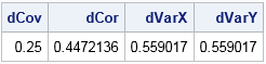
Let's test the DistCorr function on two 4-element vectors. The following (X,Y) ordered pairs lie one the intersection of the unit circle and the coordinate axes. The Pearson correlation for these observations is 0 because there is no linear association. In contrast, the distance-based correlation is nonzero. The distance correlation detects a relationship between these points (namely, that they lie along the unit circle) and therefore the variables are not independent.

x = {1,0,-1, 0};
y = {0,1, 0,-1};
results = DistCorr(x, y);
/* get itenms from results */
dCov=results$"dCov";  dCor=results$"dCor";  dVarX=results$"dVarX"; dVarY=results$"dVarY";
/* or from vector: dCov=results[1];  dCor=results[2];  dVarX=results[3]; dVarY=results[4]; */
print dCov dCor dVarX dVarY;

Examples of distance correlations

Let's look at a few other examples of distance correlations in simulated data. To make it easier to compare the Pearson correlation and the distance correlation, you can define two helper functions that return only those quantities.

Classic example: Y is quadratic function of X

The first example is the classic example (mentioned in the first paragraph of this article) that shows that a Pearson correlation of 0 does not imply independence of variables. The vector X is distributed in [-1,1] and the vector Y is defined as X²:

/* helper functions */
start PearsonCorr(x,y);
   return( corr(x||y)[1,2] );
finish;
start DCorr(x,y);
   results = DistCorr(X, Y);
   return( results$"dCor" );  /* if DistCorr returns vector: return( results[2] ); */
finish;
 
x = do(-1, 1, 0.1)`;    /* X is in [-1, 1] */
y = x##2;               /* Y = X^2 */
PCor = PearsonCorr(x,y);
DCor = DCorr(x,y);
print PCor DCor;

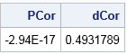
As promised, the Pearson correlation is zero but the distance correlation is nonzero. You can use the distance correlation as part of a formal hypothesis test to conclude that X and Y are not independent.

Distance correlation for multivariate normal data

You might wonder how the distance correlation compares with the Pearson correlation for bivariate normal data. Szekely et al. prove that the distance correlation is always less than the absolute value of the population parameter: dCor(X,Y) ≤ |ρ|. The following statements generate a random sample from a bivariate normal distribution with Pearson correlation ρ for a range of positive and negative ρ values.

N = 500;                   /* sample size */
mu = {0 0};  Sigma = I(2); /* parameters for bivaraite normal distrib */
rho = do(-0.9, 0.9, 0.1);  /* grid of correlations */
PCor = j(1, ncol(rho), .); /* allocate vectors for results */
DCor = j(1, ncol(rho), .);
call randseed(54321);
do i = 1 to ncol(rho);     /* for each rho, simulate bivariate normal data */
   Sigma[1,2] = rho[i]; Sigma[2,1] = rho[i]; /* population covariance */
   Z = RandNormal(N, mu, Sigma);        /* bivariate normal sample */
   PCor[i] = PearsonCorr(Z[,1], Z[,2]); /* Pearson correlation */
   DCor[i] = DCorr(Z[,1], Z[,2]);       /* distance correlation */
end;

If you graph the Pearson and distance correlation against the parameter values, you obtain the following graph:

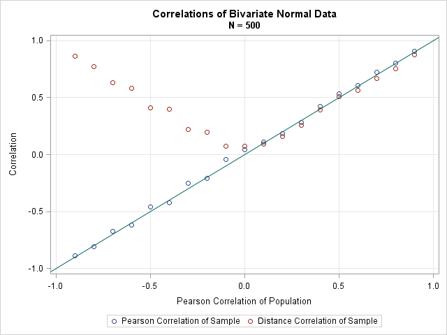
You can see that the distance correlation is always positive. It is close to, but in many cases less than, the absolute value of the Pearson estimate. Nevertheless, it is comforting that the distance correlation is closely related to the Pearson correlation for correlated normal data.

Distance correlation for data of different dimensions

As the last example, let's examine the most surprising property of the distance correlation, which is that it enables you to compute correlations between variables of different dimensions. In contrast, the Pearson correlation is defined only for univariate variables. The following statements generate two independent random normal samples with 1000 observations. The variable X is a bivariate normal sample. The variable Y is a univariate normal sample. The distance correlation for the sample is close to 0. (Because the samples were drawn independently, the distance correlation for the populations is zero.)

/* Correlation betwee a 2-D distribution and a 1-D distribution */
call randseed(12345, 1);          /* reset random number seed */
N = 1000;
mu = {0 0};
Sigma = { 1.0 -0.5, 
         -0.5  1.0};
X = RandNormal(N, mu, Sigma);     /* sample from 2-D distribution */
Y = randfun(N, "Normal", 0, 0.6); /* uncorrelated 1-D sample */
 
DCor = DCorr(X, Y);
print DCor;

Limitations of the distance correlation

The distance correlation is an intriguing idea. You can use it to test whether two variables (actually, sets of variables) are independent. As I see it, the biggest drawbacks of distance correlation are

• The distance correlation is always positive because distances are always positive. Most analysts are used to seeing negative correlations when two variables demonstrate a negative linear relationship.
• The distance correlation for a sample of size n must compute the n(n–1)/2 pairwise distances between observations. This implies that the distance correlation is an O(n²) operation, as opposed to Pearson correlation, which is a much faster O(n) operation. The implementation in this article explicitly forms the n x n distance matrix, which can become very large. For example, if n = 100,000 observations, each distance matrix requires more than 74 GB of RAM. There are ways to use less memory, but the distance correlation is still a relatively expensive computation.

Summary

In summary, this article discusses the Szekely-Rizzo-Bakirov distance-based covariance and correlation. The distance correlation can be used to create a statistical test of independence between two variables or sets of variables. The idea is interesting and appealing for small data sets. Unfortunately, the performance of the algorithm is quadratic in the number of observations, so the algorithm does not scale well to big data.

You can download the SAS/IML program that creates the computations and graphs in this article. If you do not have SAS/IML, T. Billings (2016) wrote a SAS macro that uses PROC DISTANCE to compute the distance correlation between two vectors. Rizzo and Szekely implemented their method in the 'energy' package of the R software product.