A SAS customer asked a great question: "I have parameter estimates for a logistic regression model that I computed by using multiple imputations. How do I use these parameter estimates to score new observations and to visualize the model? PROC LOGISTIC can do the computation I want, but how do I tell it to use the externally computed estimates?"

This article presents a solution for PROC LOGISTIC. At the end of this article, I present a few tips for other SAS procedures.

Here's the main idea: PROC LOGISTIC supports an INEST= option that you can use to specify initial values of the parameters. It also supports the MAXITER=0 option on the MODEL statement, which tells the procedure not to perform any iterations to try to improve the parameter estimates. When used together, you can get PROC LOGISTIC to evaluate any logistic model you want. Furthermore, you can use the STORE statement to store the model and use PROC PLM to perform scoring, visualization, and other post-fitting analyses.

I have used this technique previously to compute parameter estimates in PROC HPLOGISTIC and use them in PROC LOGISTIC to estimate odds ratios, the covariance matrix of the parameters, and other inferential quantities that are not available in PROC HPLOGISTIC. In a similar way, PROC LOGISTIC can construct ROC curves for predictions that were made outside of PROC LOGISTIC.

Produce parameter estimates by using PROC MIANALYZE

As a motivating example, let's create parameter estimates by using multiple imputations. The documentation for PROC MIANALYZE has an example of using PROC MI and PROC MIANALYZE to estimate the parameters for a logistic model. The following data and analysis are from that example. The data are lengths and widths of two species of fish (perch and parkki). Missing values are artificially introduced. A scatter plot of the data is shown.

data Fish2;
   title 'Fish Measurement Data';
   input Species $ Length Width @@;
   datalines;
Parkki  16.5  2.3265    Parkki  17.4  2.3142    .      19.8   .
Parkki  21.3  2.9181    Parkki  22.4  3.2928    .      23.2  3.2944
Parkki  23.2  3.4104    Parkki  24.1  3.1571    .      25.8  3.6636
Parkki  28.0  4.1440    Parkki  29.0  4.2340    Perch   8.8  1.4080
.       14.7  1.9992    Perch   16.0  2.4320    Perch  17.2  2.6316
Perch   18.5  2.9415    Perch   19.2  3.3216    .      19.4   .
Perch   20.2  3.0502    Perch   20.8  3.0368    Perch  21.0  2.7720
Perch   22.5  3.5550    Perch   22.5  3.3075    .      22.5   .
Perch   22.8  3.5340    .       23.5   .        Perch  23.5  3.5250
Perch   23.5  3.5250    Perch   23.5  3.5250    Perch  23.5  3.9950
.       24.0   .        Perch   24.0  3.6240    Perch  24.2  3.6300
Perch   24.5  3.6260    Perch   25.0  3.7250    .      25.5  3.7230
Perch   25.5  3.8250    Perch   26.2  4.1658    Perch  26.5  3.6835
.       27.0  4.2390    Perch   28.0  4.1440    Perch  28.7  5.1373
.       28.9  4.3350    .       28.9   .        .      28.9  4.5662
Perch   29.4  4.2042    Perch   30.1  4.6354    Perch  31.6  4.7716
Perch   34.0  6.0180    .       36.5  6.3875    .      37.3  7.7957
.       39.0   .        .       38.3   .        Perch  39.4  6.2646
Perch   39.3  6.3666    Perch   41.4  7.4934    Perch  41.4  6.0030
Perch   41.3  7.3514    .       42.3   .        Perch  42.5  7.2250
Perch   42.4  7.4624    Perch   42.5  6.6300    Perch  44.6  6.8684
Perch   45.2  7.2772    Perch   45.5  7.4165    Perch  46.0  8.1420
Perch   46.6  7.5958
;
 
proc format;
value $FishFmt
    " " = "Unknown";
run;
 
proc sgplot data=Fish2;
   format Species $FishFmt.;
   styleattrs DATACONTRASTCOLORS=(DarkRed LightPink DarkBlue);
   scatter x=Length y=Width / group=Species markerattrs=(symbol=CircleFilled);
run;

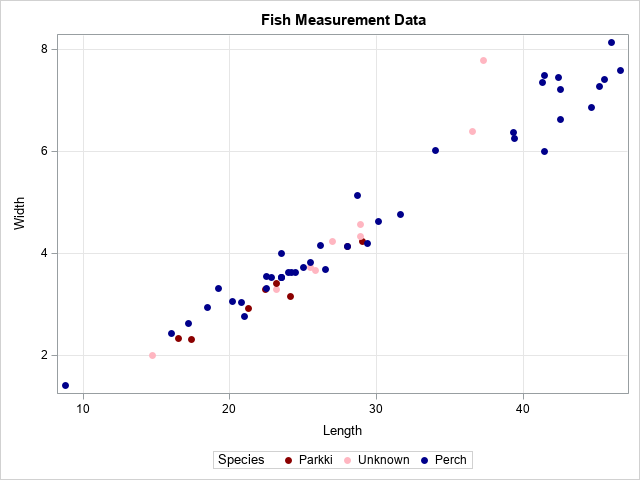
The analyst wants to use PROC LOGISTIC to create a model that uses Length and Width to predict whether a fish is perch or parkki. The scatter plot shows that the parkki (dark red) tend to be less wide than the perch of the same length For a fish of a given length, wider fish are predicted to be perch (blue) and thinner fish are predicted to be parkki (red). For some fish in the graph, the species is not known.

Because the data contains missing values, the analyst uses PROC MI to run 25 missing value imputations, uses PROC LOGISTIC to produce 25 sets of parameter estimates, and uses PROC MI to combine the estimates into a single set of parameter estimates. See the documentation for a discussion.

/* Example from the MIANALYZE documentation 
   "Reading Logistic Model Results from a PARMS= Data Set"  https://bit.ly/394VlI7
*/
proc mi data=Fish2 seed=1305417 out=outfish2;
   class Species;
   monotone logistic( Species= Length Width);
   var Length Width Species;
run;
 
ods select none; options nonotes;
proc logistic data=outfish2;
   class Species;
   model Species= Length Width / covb;
   by _Imputation_;
   ods output ParameterEstimates=lgsparms;
run;
ods select all; options notes;
 
proc mianalyze parms=lgsparms;
   modeleffects Intercept Length Width;
   ods output ParameterEstimates=MI_PE;
run;
 
proc print data=MI_PE noobs; 
  var Parm Estimate;
run;

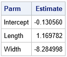
The parameter estimates from PROC MIANALYZE are shown. The question is: How can you use PROC LOGISTIC and PROC PLM to score and visualize this model, given that the estimates are produced outside of PROC LOGISTIC?

Get PROC LOGISTIC to use external estimates

As mentioned earlier, a solution to this problem is to use the INEST= option on the PROC LOGISTIC statement in conjunction with the MAXITER=0 option on the MODEL statement. When used together, you can get PROC LOGISTIC to evaluate any logistic model you want, and you can use the STORE statement to create an item store that can be read by PROC PLM to perform scoring and visualization.

You can create the INEST= data set by hand, but it is easier to use PROC LOGISTIC to create an OUTEST= data set and then merely change the values for the parameter estimates, as done in the following example:

/* 1. Use PROC LOGISTIC to create an OUTEST= data set */
proc logistic data=Fish2 outest=OutEst noprint;
   class Species;
   model Species= Length Width;
run;
 
/* 2. replace the values of the parameter estimates with different values */
data inEst;
set outEst;
Intercept = -0.130560;
Length = 1.169782;
Width = -8.284998;
run;
 
/* 3. Use the INEST= data set and MAXITER=0 to get PROC LOGISTIC to create
      a model. Use the STORE statement to write an item store.
      https://blogs.sas.com/content/iml/2019/06/26/logistic-estimates-from-hplogistic.html
*/
proc logistic data=Fish2 inest=InEst;        /* read in extermal model */
   model Species= Length Width / maxiter=0;  /* do not refine model fit */
   effectplot contour / ilink;
   store LogiModel;
run;

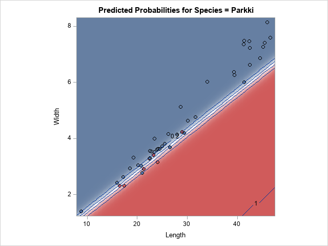
The contour plot is part of the output from PROC LOGISTIC. You could also request an ROC curve, odds ratios, and other statistics. The contour plot visualizes the regression model. For a fish of a given length, wider fish are predicted to be perch (blue) and thinner fish are predicted to be parkki (red).

Scoring the model

Because PROC LOGISTIC writes an item store for the model, you can use PROC PLM to perform a variety of scoring tasks, visualization, and hypothesis tests. The following statements create a scoring data set and use PROC PLM to score the model and estimate the probability that each fish is a parkki:

/* 4. create a score data set */
data NewFish;
input Length Width;
datalines;
17.0  2.7
18.1  2.1
21.3  2.9
22.4  3.0
29.1  4.3
;
 
/* 5. predictions on the DATA scale */
proc plm restore=LogiModel noprint;
   score data=NewFish out=ScoreILink
         predicted lclm uclm / ilink; /* ILINK gives probabilities */
run;
 
proc print data=ScoreILink; run;

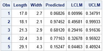
According to the model, the first and fifth fish are probably perch. The second, third, and fourth fish are predicted to be parkki, although the 95% confidence intervals indicate that you should not be too confident in the predictions for the third and fourth observations.

Thoughts on other regression procedures

Unfortunately, not every regression procedure in SAS is as flexible as PROC LOGISTIC. In many cases, it might be difficult or impossible to "trick" a SAS regression procedure into analyzing a model that was produced externally. Here are a few thoughts from me and from one of my colleagues. I didn't have time to fully investigate these ideas, so caveat emptor!

• For least squares models, the venerable PROC SCORE can handle the scoring. It can read an OUTEST/INEST-style data set, just like in the PROC LOGISTIC example. If you have CLASS variables or other constructed effects (for example, spline effects), you will have to use columns of a design matrix as variables.
• Many SAS regression procedures support the CODE statement, which writes DATA step code to score the model. Because the CODE statement writes a text file, you can edit the text file and replace the parameter estimates in the file with different estimates. However, the CODE statement does not handle constructed effects.
• The MODEL statement of PROC GENMOD supports the INITIAL= and INTERCEPT= options. Therefore, you ought to be able to specify the initial values for parameter estimates. PROC GENMOD also supports the MAXITER=0 option. Be aware that the values on the INITIAL= option must match the order that the estimates appear in the ParameterEstimates table.
• Some nonlinear modeling procedures (such as PROC NLIN and PROC NLMIXED) support ways to specify the initial values for parameters. If you specify TECH=NONE, then the procedure does not perform any optimization. These procedures also support the MAXITER= option.

Summary

This article shows how to score parametric regression models when the parameter estimates are not fit by the usual procedures. For example, multiple imputations can produce a set of parameter estimates. In PROC LOGISTIC, you can use an INEST= data set to read the estimates and use the MAXITER=0 option to suppress fitting. You can use the STORE statement to store the model and use PROC PLM to perform scoring and visualization. Other procedures have similar options, but there is not a single method that works for all SAS regression procedures.

If you use any of the ideas in this article, let me know how they work by leaving a comment. If you have an alternate way to trick SAS regression procedures into using externally supplied estimates, let me know that as well.