When there are two equivalent ways to do something, I advocate choosing the one that is simpler and more efficient. Sometimes, I encounter a SAS program that simulates random numbers in a way that is neither simple nor efficient. This article demonstrates two improvements that you can make to your SAS code if you are simulating binary variables or categorical variables.

Simulate a random binary variable

The following DATA step simulates N random binary (0 or 1) values for the X variable. The probability of generating a 1 is p=0.6 and the probability of generating a 0 is 0.4. Can you think of ways that this program can be simplified and improved?

%let N = 8;
%let seed = 54321;
 
data Binary1(drop=p);
call streaminit(&seed);
p = 0.6;
do i = 1 to &N;
   u = rand("Uniform");
   if (u < p) then
      x=1;
   else
      x=0;
   output;
end;
run;
 
proc print data=Binary1 noobs; run;

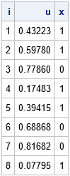
The goal is to generate a 1 or a 0 for X. To accomplish this, the program generates a random uniform variate, u, which is in the interval (0, 1). If u < p, it assigns the value 1, otherwise it assigns the value 0.

Although the program is mathematically correct, the program can be simplified. It is not necessary for this program to generate and store the u variable. Yes, you can use the DROP statement to prevent the variable from appearing in the output data set, but a simpler way is to use the Bernoulli distribution to generate X directly. The Bernoulli(p) distribution generates a 1 with probability p and generates a 0 with probability 1-p. Thus, the following DATA step is equivalent to the first, but is both simpler and more efficient. Both programs generate the same random binary values.

data Binary2(drop=p);
call streaminit(&seed);
p = 0.6;
do i = 1 to &N;
   x = rand("Bernoulli", p);     /* Bern(p) returns 1  with probability p */
   output;
end;
run;
 
proc print data=Binary2 noobs; run;

Simulate a random categorical variable

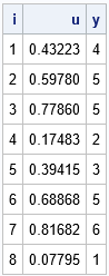
The following DATA step simulates N random categorical values for the X variable. If p = {0.1, 0.1, 0.2, 0.1, 0.3, 0.2} is a vector of probabilities, then the probability of generating the value i is p[i]. For example, the probability of generating a 3 is 0.2. Again, the program generates a random uniform variate and uses the cumulative probabilities ({0.1, 0.2, 0.4, 0.5, 0.8, 1}) as cutpoints to determine what value to assign to X, based on the value of u. (This is called the inverse CDF method.)

/* p = {0.1, 0.1, 0.2, 0.1, 0.3, 0.2} */
/* Use the cumulative probability as cutpoints for assigning values to X */
%let c1 = 0.1;
%let c2 = 0.2;
%let c3 = 0.4;
%let c4 = 0.5;
%let c5 = 0.8;
%let c6 = 1;
 
data Categorical1;
call streaminit(&seed);
do i = 1 to &N;
   u = rand("Uniform");
   if (u <=&c1) then
      y=1;
   else if (u <=&c2) then
      y=2;
   else if (u <=&c3) then
      y=3;
   else if (u <=&c4) then
      y=4;
   else if (u <=&c5) then
      y=5;
   else
      y=6;
   output;
end;
run;
 
proc print data=Categorical1 noobs; run;

If you want to generate more than six categories, this indirect method becomes untenable. Suppose you want to generate a categorical variable that has 100 categories. Do you really want to use a super-long IF-THEN/ELSE statement to assign the values of X based on some uniform variate, u? Of course not! Just as you can use the Bernoulli distribution to directly generate a random variable that has two levels, you can use the Table distribution to directly generate a random variable that has k levels, as follows:

data Categorical2;
call streaminit(&seed);
array p[6] _temporary_ (0.1, 0.1, 0.2, 0.1, 0.3, 0.2);
do i = 1 to &N;
   x = rand("Table", of p[*]); /* Table(p) returns i with probability p[i] */
   output;
end;
 
proc print data=Categorical2 noobs; run;

Summary

In summary, this article shows two tips for simulating discrete random variables:

1. Use the Bernoulli distribution to generate random binary variates.
2. Use the Table distribution to generate random categorical variates.

These distributions enable you to directly generate categorical values based on supplied probabilities. They are more efficient than the oft-used method of assigning values based on a uniform random variate.