During an epidemic, such as the coronavirus pandemic of 2020, the media often shows graphs of the cumulative numbers of confirmed cases for different countries. Often these graphs use a logarithmic scale for the vertical axis. In these graphs, a straight line indicates that new cases are increasing at an exponential rate. The slope of the line indicates how quickly cases will double, with steep lines indicating a short doubling time. The doubling time is the length of time required to double the number of confirmed cases, assuming nothing changes.

This article shows one way to estimate the doubling time by using the most recent data. The method uses linear regression to estimate the slope (m) of a curve, then estimates the doubling time as log(2) / m.

The data in this article are the cumulative counts for COVID-19 cases in four countries (Italy, the United States, Canada, and South Korea) for the dates 03Mar2020 to 27Mar2020. You can download the data and SAS program for this article.

A log-scale visualization of the cumulative cases

The data set contains four variables:

• The Region variable specifies the country.
• The Day variable specifies the number of days since 03Mar2020.
• The Cumul variable specifies the cumulative counts of confirmed cases of COVID-19.
• The Log10Cumul variable specifies the base-10 logarithm of the confirmed cases. In SAS, you can use the LOG10 function to compute the base-10 logarithm.

You can use PROC SGPLOT to visualize these data. The following graph plots the total number of cases, but uses the TYPE=LOG and LOGBASE=10 options to specify a base-10 logarithmic axis for the counts:

title "Cumulative Counts (log scale)";
proc sgplot data=Virus;
  where Cumul > 0;
  series x=Day y=Cumul / group=Region curvelabel;
  xaxis grid;
  yaxis type=LOG logbase=10 grid
        values=(100 500 1000 5000 10000 50000 100000) ValuesHint;
run;

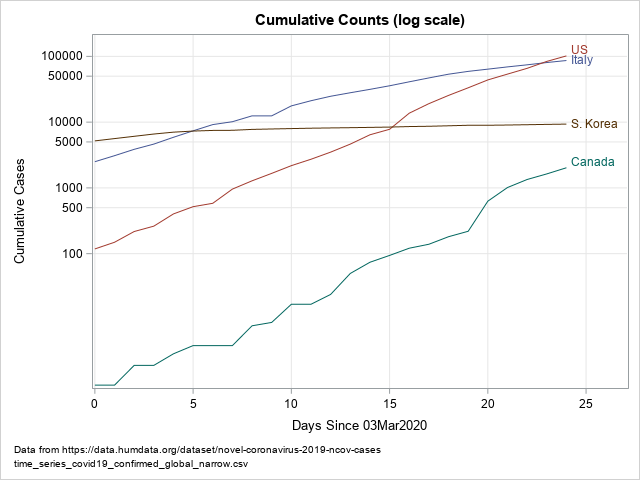
This graph is sometimes called a semi-log graph because only one axis is displayed on a log scale. A straight line on a semi-log graph indicates exponential growth. However, all exponential growth is not equal. The slope of the line indicates how quickly the growth is occurring, and the doubling time is one way to measure the growth. A line with a steep slope indicates that the underlying quantity (confirmed cases) will double in a short period of time. A line with a flat slope indicates that the underlying quantity is not growing as quickly and will take a long time to double. For these data, the visualization reveals the following facts:

• The curves for the United States and Canada have steep slopes.
• The curve for South Korea is much flatter, which indicates that the number of confirmed cases is growing very slowly in that country.
• The slope of the curve for Italy looks similar to the US curve for days 0–6, but then the Italy curve begins to flatten. Although the US and Italy had the same number of cases on Day 24, the slope of the Italy curve was less than the slope of the US curve. The interpretation is that (on Day 24) the estimated doubling time for US cases is shorter than for Italy.

An estimate of the slope at the end of each curve

Some researchers fit a linear regression to all values on the curve in order to estimate an average slope. This is usually not a good idea because interventions (such as stay-at-home orders) cause the curves to bend over time. This is clearly seen in the curves for Italy and South Korea.

You can get a better estimate for the current rate of growth if you fit a regression line by using only recent data values. I suggest using data from several previous days, such as the previous 5 or 7 days. You can use the REG procedure in SAS to estimate the slope of each line based on the five most recent observations:

%let MaxDay = 24;
proc reg data=Virus outest=Est noprint;
  where Day >= %eval(&MaxDay-4);           *previous 5 days: Day 20, 21, 22, 23, and 24;
  by Region notsorted;
  model log10Cumul = Day;
quit;

The Est data set contains estimates of the slope (and intercept) for the line that best fits the recent data. The estimates are shown in a subsequent section.

An estimate of the doubling time

You can use these estimated slopes to estimate the doubling time for each curve. If a quantity Y increases from Y₀ at time t₀ to 2*Y₀ at some future time t₀ + Δt, the value Δt is the doubling time. The next paragraph shows that the doubling time at t₀ is log(2) / m, where m is an estimate of the slope at t₀.

The idea is to use the tangent line at t₀ to estimate the doubling time. Let log(Y) = m*t + b be the equation of the tangent line at t₀ on the semi-log graph. When Y increases from Y₀ to 2*Y₀, the logarithm increases from log(Y₀) to log(2*Y₀) = log(2)+log(Y₀). Since the slope is "rise over run," the tangent line reaches the doubled value when
m = [(log(2) + log(Y₀)) - log(Y₀)] / Δt = log(2) / Δt.
Solving for Δt gives
Δt = log(2) / m,
where m is the slope of a regression line for the semi-log curve at t₀. This formula estimates the doubling time, which does not depend on the value of Y, only on the slope at t₀.

Estimate the doubling time from the slope

The following SAS DATA step estimates the doubling time by using the slope estimates at the end of each curve (Day 24):

data DoublingTime;
set Est(rename=(Day=Slope));
label Slope = "Slope of Line" DoublingTime = "Doubling Time";
DoublingTime = log10(2) / Slope;
keep Region Intercept Slope DoublingTime;
run;
 
proc print data=DoublingTime label noobs;
  format Slope DoublingTime 6.3;
  var Region Slope DoublingTime;
run;

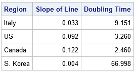
For a pandemic, short doubling times are bad and long doubling times are good. Based on the 27Mar2020 data, the table estimates the doubling time for Italy to be 9 days. In contrast, the estimate for the US doubling time is about 3.3 days, and the estimate for Canada is about 2.5. The estimate for South Korea is 67 days, but for such a long time period the assumption that "the situation stays the same" is surely not valid.

Visualizing the doubling time

You can visualize the doubling times by adding an arrow to the end of each curve:

• The base of the arrow is located at the most recent data.
• The direction of the arrow is determined by the estimated slope of the curve.
• The horizontal extent of the arrow is the doubling time.
• The vertical extent of the arrow is twice the current count.

The arrows are shown in the following visualization, which excludes South Korea:

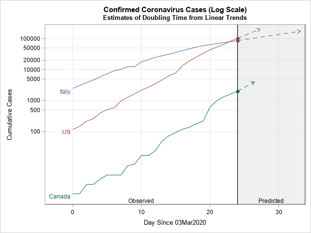
This graph shows how quickly the US and Canadian counts are predicted to double. The tip of each arrow indicates the time at which the number of cases are predicted to double. For the US and Canada, this is only a few days. The arrow for Italy indicates a longer time before the Italian cases double. Again, these calculations assume that the number of cases continues to grow at the estimated rate on Day 24. Because the curve for Italy appears to be flattening, the Italian estimate will (hopefully) be overly pessimistic.

Summary

In summary, you can use the slope of a cumulative curve (on a log scale) to estimate the doubling time for the underlying quantity. To find the slope at the most recent observation, you can fit a linear regression line to recent data. The doubling time is given by log(2)/m, where m is the estimate of the slope of the cumulative curve in a semi-log graph. If you want to visualize the doubling time on the graph, you can add an arrow to the end of each curve.