In a linear regression model, the predicted values are on the same scale as the response variable. You can plot the observed and predicted responses to visualize how well the model agrees with the data, However, for generalized linear models, there is a potential source of confusion. Recall that a generalized linear model (GLIM) has two components: a linear predictor, which is a linear combination of the explanatory variables, and a transformation (called the inverse link function) that maps the linear predictor onto the scale of the data. Consequently, SAS regression procedures support two types of predicted values and prediction limits. In the SAS documentation, the first type is called "predictions on the linear scale" whereas the second type is called "predictions on the data scale."

For many SAS procedures, the default is to compute predicted values on the linear scale. However, for GLIMs that model nonnormal response variables, it is more intuitive to predict on the data scale. The ILINK option, which is shorthand for "apply the inverse link transformation," converts the predicted values to the data scale. This article shows how the ILINK option works by providing an example for a logistic regression model, which is the most familiar generalized linear models.

Review of generalized linear models

The SAS documentation provides an overview of GLIMs and link functions. The documentation for PROC GENMOD provides a list of link functions for common regression models, including logistic regression, Poisson regression, and negative binomial regression.

Briefly, the linear predictor is
η = X*β
where X is the design matrix and β is the vector of regression coefficients. The link function (g) is a monotonic function that relates the linear predictor to the conditional mean of the response. Sometimes the symbol μ is used to denote the conditional mean of the response (μ = E[Y|x]), which leads to the formula
g(μ) = X*β

In SAS, you will often see options and variables names (in output data sets) that contains the substring 'XBETA'. When you see 'XBETA', it indicates that the statistic or variable is related to the LINEAR predictor. Because the link function, g, is monotonic, it has an inverse, g^-1. For generalized linear models, the inverse link function maps the linear-scale predictions to data-scale predictions: if η = x β is a predicted value on the linear scale, then g^-1(η) is the predicted value for x on the data scale.

When the response variable is binary, the GLIM is the logistic model. If you use the convention that Y=1 indicates an event and Y=0 indicates the absence of an event, then the "data scale" is [0, 1] and the GLIM predicts the probability that the event occurs. For the logistic GLIM, the link function is the logit function:
g(μ) = logit(μ) = log( μ / (1 - μ) )
The inverse of the logit function is called the logistic function:
g^-1(η) = logistic(η) = 1 / (1 + exp(-η))

To demonstrate the ILINK option, the next sections perform the following tasks:

1. Use PROC LOGISTIC to fit a logistic model to data. You can use the STORE statement to store the model to an item store.
2. Use the SCORE statement in PROC PLM to score new data. This example scores data by using the ILINK option.
3. Score the data again, but this time do not use the ILINK option. Apply the logistic transformation to the linear estimates to demonstrate that relationship between the linear scale and the data scale.

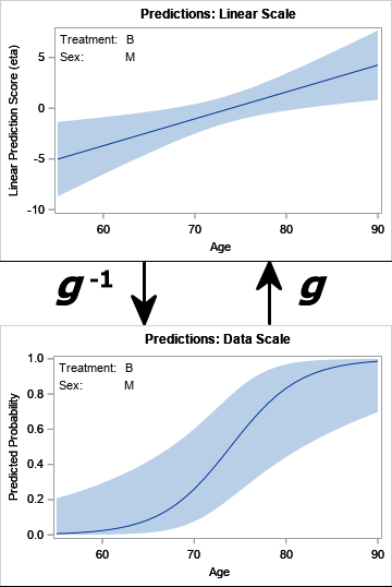
The transformation between the linear scale and the data scale is illustrated by the following graph:

Fit a logistic model

The following data are from the documentation for PROC LOGISTIC. The model predicts the probability of Pain="Yes" (the event) for patients in a study, based on the patients' sex, age, and treatment method ('A', 'B', or 'P'). The STORE statement in PROC LOGISTIC creates an item store that can be used for many purposes, including scoring new observations.

data Neuralgia;
   input Treatment $ Sex $ Age Duration Pain $ @@;
   DROP Duration;
   datalines;
P F 68  1 No  B M 74 16 No  P F 67 30 No  P M 66 26 Yes B F 67 28 No  B F 77 16 No
A F 71 12 No  B F 72 50 No  B F 76  9 Yes A M 71 17 Yes A F 63 27 No  A F 69 18 Yes
B F 66 12 No  A M 62 42 No  P F 64  1 Yes A F 64 17 No  P M 74  4 No  A F 72 25 No
P M 70  1 Yes B M 66 19 No  B M 59 29 No  A F 64 30 No  A M 70 28 No  A M 69  1 No
B F 78  1 No  P M 83  1 Yes B F 69 42 No  B M 75 30 Yes P M 77 29 Yes P F 79 20 Yes
A M 70 12 No  A F 69 12 No  B F 65 14 No  B M 70  1 No  B M 67 23 No  A M 76 25 Yes
P M 78 12 Yes B M 77  1 Yes B F 69 24 No  P M 66  4 Yes P F 65 29 No  P M 60 26 Yes
A M 78 15 Yes B M 75 21 Yes A F 67 11 No  P F 72 27 No  P F 70 13 Yes A M 75  6 Yes
B F 65  7 No  P F 68 27 Yes P M 68 11 Yes P M 67 17 Yes B M 70 22 No  A M 65 15 No
P F 67  1 Yes A M 67 10 No  P F 72 11 Yes A F 74  1 No  B M 80 21 Yes A F 69  3 No
;
 
title 'Logistic Model on Neuralgia';
proc logistic data=Neuralgia;
   class Sex Treatment;
   model Pain(Event='Yes')= Sex Age Treatment;
   store PainModel / label='Neuralgia Study';  /* store model for post-fit analysis */
run;

Score new data by using the ILINK option

There are many reasons to use PROC PLM, but an important purpose of PROC PLM is to score new observations. Given information about new patients, you can use PROC PLM to predict the probability of pain if these patients are given a specific treatment. The following DATA step defines the characteristics of four patients who will receive Treatment B. The call to PROC PLM scores and uses the ILINK option to predict the probability of pain:

/* Use PLM to score new patients */
data NewPatients;
   input Treatment $ Sex $ Age Duration;
   DROP Duration;
   datalines;
B M 67 15 
B F 73  5 
B M 74 12 
B F 79 16 
;
 
/* predictions on the DATA scale */
proc plm restore=PainModel noprint;
   score data=NewPatients out=ScoreILink
         predicted lclm uclm / ilink; /* ILINK gives probabilities */
run;
 
proc print data=ScoreILink; run;

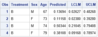
The Predicted column contains probabilities in the interval [0, 1]. The 95% prediction limits for the predictions are given by the LCLM and UCLM columns. For example, the prediction interval for the 67-year-old man is approximately [0.03, 0.48].

These values and intervals are transformations of analogous quantities on the linear scale. The logit transformation maps the predicted probabilities to the linear estimates. The inverse logit (logistic) transformation maps the linear estimates to the predicted probabilities.

Linear estimates and the logistic transformation

The linear scale is important because effects are additive on this scale. If you are testing the difference of means between groups, the tests are performed on the linear scale. For example, the ESTIMATE, LSMEANS, and LSMESTIMATE statements in SAS perform hypothesis testing on the linear estimates. Each of these statements supports the ILINK option, which enables you to display predicted values on the data scale.

To demonstrate the connection between the predicted values on the linear and data scale, the following call to PROC PLM scores the same data according to the same model. However, this time the ILINK option is omitted, so the predictions are on the linear scale.

/* predictions on the LINEAR scale */
proc plm restore=PainModel noprint;
   score data=NewPatients out=ScoreXBeta(
         rename=(Predicted=XBeta LCLM=LowerXB UCLM=UpperXB))
         predicted lclm uclm;         /* ILINK not used, so linear predictor */
run;
 
proc print data=ScoreXBeta; run;

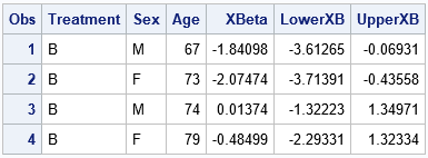
I have renamed the variables that PROC PLM creates for the estimates on the linear scale. The XBeta column shows the predicted values. The LowerXB and UpperXB columns show the prediction interval for each patient. The XBeta column shows the values you would obtain if you use the parameter estimates table from PROC LOGISTIC and apply those estimates to the observations in the NewPatients data.

To demonstrate that the linear estimates are related to the estimates in the previous section, the following SAS DATA step uses the logistic (inverse logit) transformation to convert the linear estimates onto the predicted probabilities:

/* Use the logistic (inverse logit) to transform the linear estimates
     (XBeta) into probability estimates in [0,1], which is the data scale.
   You can use the logit transformation to go the other way. */
data LinearToData;
   set ScoreXBeta;   /* predictions on linear scale */
   PredProb   = logistic(XBeta);
   LCLProb    = logistic(LowerXB);
   UCLProb    = logistic(UpperXB); 
run;
 
proc print data=LinearToData;
   var Treatment Sex Age PredProb LCLProb UCLProb;
run;

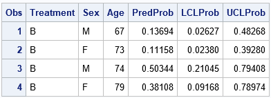
The transformation of the linear estimates gives the same values as the estimates that were obtained by using the ILINK option in the previous section.

Summary

In summary, there are two different scales for predicting values for a generalized linear model. When you report predicted values, it is important to specify the scale you are using. The data scale makes intuitive sense because it is the same scale as the response variable. You can use the ILINK option in SAS to get predicted values and prediction intervals on the data scale.