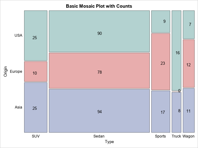
Find the center of each cell in a mosaic plot

I recently showed how to create an annotation data set that will overlay cell counts or percentages on a mosaic plot. A mosaic plot is a visual representation of a cross-tabulation of observed frequencies for two categorical variables. The mosaic plot with cell counts is shown to the right. The previous article focused on how to create the mosaic plot and how to apply an annotation, assuming that the centers of each cell were provided. This article shows how to compute the center of the cells from the output of PROC FREQ.

A motivating example

In a two-way mosaic plot, the widths of the bars represent the proportions of the levels of the categorical variables. It makes sense, therefore, to use [0, 100] as the coordinate system for the mosaic plots. For example, suppose the horizontal variable has three levels (A, B, and C) and the proportion of A is 20%, the proportion of B is 30%, and the proportion of C is 50%. Then the widths of the bars in the coordinate system are 20, 30, and 50, respectively. The first bar covers the range [0, 20], the second bar covers [20, 50], and the third bar covers [50, 100]. The widths of the bars will occupy 20%, 30%, and 50% of the width of the mosaic plot. In general, if the widths of the bars are w1, w2, and w3, the bars cover the intervals [0, w1], [w1, w1+w2], and [w1+w2, 100]. The centers of the bars are at w1/2, w1 + w2/2, and w1 + w2 + w3/2, respectively.

Each bar is composed of smaller vertical bars. If you adopt a [0, 100] coordinate system for the vertical dimension, the heights of the sub-bars are the conditional proportions of the vertical variable within each level of the horizontal variable.

Obtain the proportions and conditional proportions from PROC FREQ

You can use PROC FREQ to obtain the proportions of each level and joint level. You can use the proportions to compute the center of each cell in a [0, 100] x [0, 100] coordinate system. I recommend using the CROSSLIST and SPARSE options, as shown in the following example, which shows a mosaic plot for the Origin and Type variables in the Sashelp.Cars data. For portability (and, hopefully, clarity), I have defined two macros that contain the name of the horizontal and vertical variables.

%let hVar = Type;             /* name of horizontal variable */
%let vVar = Origin;           /* name of vertical variable */
 
proc freq data=Sashelp.Cars;
   where Type ^= 'Hybrid';
   tables &vVar * &hVar / crosslist sparse 
                          out=FreqOut(where=(Percent^=.));
   ods output CrossList=FreqList;    /* output CROSSLIST table */
run;

The CROSSLIST option creates a data set where the formatted values of the horizontal and vertical variables (Origin and Type, respectively) begin with the prefix "F_", which stands for "formatted values." These are always character variables. You can use WHERE clauses to subset the data that you need to compute the centers of the mosaic cells:

When F_Origin equals "Total," the Frequency and Percent variables contain the information you need to compute the width of the mosaic bars.
The other rows contain the information needed to compute the heights of the bars for each stacked bar. The ColPercent variable contains the conditional proportions for each bar.

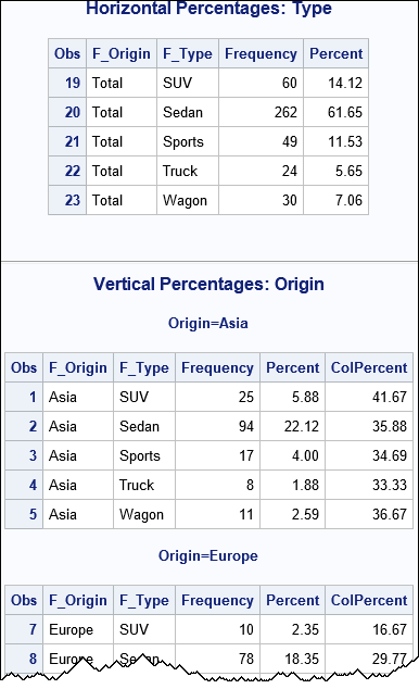
The following PROC PRINT statements show the relevant information for this example:

title "Horizontal Percentages: &hVar";
proc print data=FreqList;
   where F_&vVar='Total' & F_&hVar^='Total';
   var F_&vVar F_&hVar Frequency Percent;
run;
 
title "Vertical Percentages: &vVar";
proc print data=FreqList;
   where F_&vVar ^= 'Total' & F_&hVar ^= 'Total';
   by F_&vVar notsorted;
   var F_&vVar F_&hVar Frequency Percent ColPercent;
run;

Find the centers of each cell

As shown in the previous section, the FreqList data set contains all the information you need to find the center of each cell in the mosaic plot. Mathematically, it is not hard to convert that information into the coordinates of the cell centers. Programmatically, the process is complicated. The following SAS/IML program computes the centers by using the following steps:

Read the percentages for the levels of the horizontal variable.
Use these and the CUSUM function to find the horizontal centers of the bars.
For each level of the horizontal variable, read the percentages for the levels of the vertical variable.
Use these to find the vertical centers of each stacked bar.
Write this information to a SAS data set in the long form. Include the observed frequencies and percentages for each cell.

/* Read CROSSLIST data set and write data set that contains centers of cells in mosaic plot.
  Main idea: If a categorical variable has three levels and observed proportions are
  20, 30, and 50, then the midpoints of the bars are
       10 = 20/2
       35 = 20 + 30/2
       75 = 20 + 30 + 50/2
*/
proc iml;
/* 1. read percentages for the horizontal variable */
use FreqList;
read all var {Percent F_&hVar F_&vVar}
         where (F_&vVar='Total' & F_&hVar^='Total');
hPos = Percent;            
nH = nrow(hPos);
hLabel = F_&hVar;
 
/* 2. horizontal centers
   h1/2,  h1 + h2/2, h1 + h2 + h3/2, h1 + h2 + h3 + h4/2, ... */
halfW = hPos / 2;
hCenter = halfW + cusum(0 // hPos[1:(nH-1)]);
print (hCenter`)[c=hLabel L="hCenter" F=5.2];
 
/* 3. For each column, read cell percentages and frequencies */
read all var {Frequency Percent ColPercent F_&vVar F_&hVar}
     where (F_&vVar^='Total' &  F_&hVar ^= 'Total');
close;
FhVar = F_&hVar;              /* levels of horiz var */
FvVar = F_&vVar;              /* lavels of vert var */
*print FhVar fVVar Frequency Percent ColPercent;
 
/* 4. Get the counts and percentages for each cell.
   Vertical centers are 
   v1/2,  v1 + v2/2, v1 + v2 + v3/2, ... */
vLabel = shape( FvVar, 0, nH )[,1];
vPos = shape( ColPercent, 0, nH );
nV = nrow(vPos);
halfW = vPos / 2;
vCenters = j(nrow(vPos), ncol(vPos), .);
do i = 1 to nH;
   vCenters[,i] = halfW[,i] + cusum(0 // vPos[1:(nV-1),i]);
end;
print vCenters[r=vLabel c=hLabel F=5.2];
 
/* 5. convert to a long format: (hPos, vPos, Freq, Pct) 
   and write to SAS data set */
hCenters = repeat(hCenter, nV);
CellFreq = shape( Frequency, 0, nH );
CellPct = shape( Percent, 0, nH );
result = colvec(hCenters) || colvec(vCenters) || 
         colvec(CellFreq) || colvec(CellPct);
*print FhVar FvVar result[c={"hCenter" "vCenter" "Freq" "Pct"}];
 
/* Optional: You might want to get rid of any labels that account to fewer 
   than 2% (or 1%) of the total. The criterion is up to you. For example: 
   idx = loc( result[,4] > 2 );  * keep if greater than 2% of total;
   result = result[idx, ];
*/
 
/* write character and numeric vars separately, then merge together */
/* Character vars: pairwise labels of horiz and vertical categories */
create labels var {FhVar FvVar}; append; close;
/* Numeric vars: centers of cells, counts, and percentages */
create centers from result[c={"hCenter" "vCenter" "Freq" "Pct"}];
   append from result;
close;
QUIT;
 
data annoData;
   merge labels centers;
run;

Convert centers into an annotation data set

The variables and values in an SG annotation data set must use special names so that the annotation facility knows how to interpret the data. For an introduction to GTL annotation, see the GTL documentation or Warren Kuhfeld's free e-book Advanced ODS Graphics Examples. To overlay text, you need to include the following information:

The Label variable specifies the text to display.
The x1 and y1 variables specify the coordinates of the label (in the LAYOUTPERCENT drawing space).
The Width variable specifies the width of the label and the Anchor variable specifies how the text is anchored (left, right, centered,...) at the (x1, y1) location.

However, as discussed in my previous article, a "region plot" such as the mosaic plot does not support the GRAPHPERCENT or WALLPERCENT drawing areas. You have to use the LAYOUTPERCENT drawing area, which includes space for the axes. Therefore, you cannot merely use the centers as the (x1, x2) coordinates. Instead, you need to linearly transform the centers so that they correctly align with the mosaic cells.

I do not know how to do this step in a general way that will accommodate all situations. You need to look at the graph (including its physical dimensions, font sizes, the length of the labels, etc.) and make a guess about how to linearly transform the center data. In the following program, I estimate that the axis area is about 10% of the horizontal and vertical portion of the layout drawing region. Therefore, I shrink the centers by 10% (that is, multiply by 0.9) and translate the result by 10%. You might need to use different values for your data.

The following statements create the annotation data step. For completeness, I've also included the statements that define the mosaic template and create the graph with the annotation.

/* If we could use the WALLPERCENT drawing space, we could
   use (hCenter, vCenter) as the drawing coordinates:
   x1 = hCenter;
   y1 = vCenter;
 
   Unfortunately, we have to use LAYOUTPERCENT, so perform a linear
   transformation from "wall coordinates" to layout coordinates.
*/
data anno;
set AnnoData;
length label $12;
/* use RETAIN stmt to define values that are constant */
retain function 'text' 
       y1space 'layoutpercent' x1space 'layoutpercent'
       width 4        /* make larger if you are plotting percentages */
       anchor 'center';
/* Guess a linear transform to LAYOUTPERCENT coordinates.
   Need to move inside graph area, so shrink and 
   translate to correct for left and bottom axes areas */
x1 = 0.9*hCenter + 10;
y1 = 0.9*vCenter + 10;   
label = put(Freq, 5.);
run;
 
/* Note: PROC FREQ reverses Y axis b/c it sorts the FreqOut data in descending order. */
proc template;
  define statgraph mosaicPlotParm;
  dynamic _VERTVAR _HORZVAR _FREQ _TITLE;
    begingraph;
      entrytitle _TITLE;
      layout region;    /* REGION layout, so can't overlay text! */
      MosaicPlotParm category=(_HORZVAR _VERTVAR) count=_FREQ / 
             datatransparency=0.5
             colorgroup=_VERTVAR name="mosaic";
      endlayout;
      annotate;         /* required for annotation */
    endgraph;
  end;
run;
 
proc sgrender data=FreqOut template=mosaicPlotParm sganno=anno;
dynamic _VERTVAR="Origin" _HORZVAR="Type" _FREQ="Count"
        _TITLE="Basic Mosaic Plot with Counts";
run;

The mosaic plot with text annotations is shown at the top of this program.

In the previous article, I showed how you can use the GTL annotation facility to overlay frequency counts or percentages on a mosaic plot in SAS. In this article, I show how to write a program that computes the centers of the cells from the percentages that PROC FREQ provides when you use the CROSSLIST SPARSE option. Unfortunately, after you compute the centers, you cannot use them directly because the mosaic plot does not support the WALLPERCENT drawing space. Instead, you must use the LAYOUTPERCENT drawing space, which means you need to linearly transform the cell centers.

You can download the SAS program that computes the centers of mosaic cells and uses those coordinates to annotate the mosaic plot.

Blogs