A data analyst asked how to compute parameter estimates in a linear regression model when the underlying data matrix is rank deficient. This situation can occur if one of the variables in the regression is a linear combination of other variables. It also occurs when you use the GLM parameterization of a classification variable. In the GLM parameterization, the columns of the design matrix are linearly dependent. As a result, the matrix of crossproducts (the X`X matrix) is singular. In either case, you can understand the computation of the parameter estimates by learning about generalized inverses in linear systems. This article presents an overview of generalized inverses. A subsequent article will specifically apply generalized inverses to the problem of estimating parameters for regression problems with collinearities.

What is a generalized inverse?

Recall that the inverse matrix of a square matrix A is a matrix G such as A*G = G*A = I, where I is the identity matrix. When such a matrix exists, it is unique and A is said to be nonsingular (or invertible). If there are linear dependencies in the columns of A, then an inverse does not exist. However, you can define a series of weaker conditions that are known as the Penrose conditions:

1. A*G*A = A
2. G*A*G = G
3. (A*G)` = A*G
4. (G*A)` = G*A

Any matrix, G, that satisfies the first condition is called a generalized inverse (or sometimes a "G1" inverse) for A. A matrix that satisfies the first and second conditions is called a "G2" inverse for A. The G2 inverse is used in statistics to compute parameter estimates for regression problems (see Goodnight (1979), p. 155). A matrix that satisfies all four conditions is called the Moore-Penrose inverse or the pseudoinverse. When A is square but singular, there are infinitely many matrices that satisfy the first two conditions, but the Moore-Penrose inverse is unique.

Computations with generalized inverses

In regression problems, the parameter estimates are obtained by solving the "normal equations." The normal equations are the linear system (X`*X)*b = (X`*Y), where X is the design matrix, Y is the vector of observed responses, and b is the parameter estimates to be solved. The matrix A = X`*X is symmetric. If the columns of the design matrix are linearly dependent, then A is singular. The following SAS/IML program defines a symmetric singular matrix A and a right-hand-side vector c, which you can think of as X`*Y in the regression context. The call to the DET function computes the determinant of the matrix. A zero determinant indicates that A is singular and that there are infinitely many vectors b that solve the linear system:

proc iml;
A = {100  50 20 10,
      50 106 46 23,
      20  46 56 28,
      10  23 28 14 };
c = {130, 776, 486, 243};
 
det = det(A);         /* demonstrate that A is singular */
print det;

For nonsingular matrices, you can use either the INV or the SOLVE functions in SAS/IML to solve for the unique solution of the linear system. However, both functions give errors when called with a singular matrix. SAS/IML provides several ways to compute a generalized inverse, including the SWEEP function and the GINV function. The SWEEP function is an efficient way to use Gaussian elimination to solve the symmetric linear systems that arise in regression. The GINV function is a function that computes the Moore-Penrose pseudoinverse. The following SAS/IML statements compute two different solutions for the singular system A*b = c:

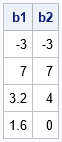
b1 = ginv(A)*c;       /* solution even if A is not full rank */
b2 = sweep(A)*c;
print b1 b2;

The SAS/IML language also provides a way to obtain any of the other infinitely many solutions to the singular system A*b = c. Because A is a rank-1 matrix, it has a one-dimensional kernel (null space). The HOMOGEN function in SAS/IML computes a basis for the null space. That is, it computes a vector that is mapped to the zero vector by A. The following statements compute the unit basis vector for the kernel. The output shows that the vector is mapped to the zero vector:

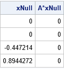
xNull = homogen(A);   /* basis for nullspace of A */
print xNull (A*xNull)[L="A*xNull"];

All solutions to A*b = c are of the form b + α*xNull, where b is any particular solution.

Properties of the Moore-Penrose solution

You can verify that the Moore-Penrose matrix GINV(A) satisfies the four Penrose conditions, whereas the G2 inverse (SWEEP(A)) only satisfies the first two conditions. I mentioned that the singular system has infinitely many solutions, but the Moore-Penrose solution (b1) is unique. It turns out that the Moore-Penrose solution is the solution that has the smallest Euclidean norm. Here is a computation of the norm for three solutions to the system A*b = c:

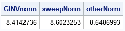
/* GINV gives the estimate that has the smallest L2 norm: */
GINVnorm  = norm(b1);
sweepNorm = norm(b2);
/* you can add alpha*xNull to any solution to get another solution */
b3 = b1 + 2*xNull;  /* here's another solution (alpha=2) */
otherNorm = norm(b3);
print ginvNorm sweepNorm otherNorm;

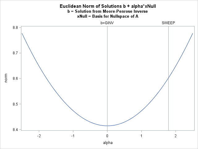
Because all solutions are of the form b1 + α*xNull, where xNull is the basis for the nullspace of A, you can graph the norm of the solutions as a function of α. The graph is shown below and indicates that the Moore-Penrose solution is the minimal-norm solution:

alpha = do(-2.5, 2.5, 0.05);
norm = j(1, ncol(alpha), .);
do i = 1 to ncol(alpha);
   norm[i] = norm(b1 + alpha[i] * xNull);
end;
title "Euclidean Norm of Solutions b + alpha*xNull";
title2 "b = Solution from Moore-Penrose Inverse";
title3 "xNull = Basis for Nullspace of A";
call series(alpha, norm) 
     other="refline 0 / axis=x label='b=GINV';refline 1.78885 / axis=x label='SWEEP';";

In summary, a singular linear system has infinitely many solutions. You can obtain a particular solution by using the sweep operator or by finding the Moore-Penrose solution. You can use the HOMOGEN function to obtain the full family of solutions. The Moore-Penrose solution is expensive to compute but has an interesting property: it is the solution that has the smallest Euclidean norm. The sweep solution is more efficient to compute and is used in SAS regression procedures such as PROC GLM to estimate parameters in models that include classification variables and use a GLM parameterization. A subsequent blog post explores regression estimates in more detail.