In a recent article about nonlinear least squares, I wrote, "you can often fit one model and use the ESTIMATE statement to estimate the parameters in a different parameterization." This article expands on that statement. It shows how to fit a model for one set of parameters and use the ESTIMATE statement to obtain estimates for a different set of parameters.

A canonical example of a probability distribution that has multiple parameterizations is the gamma distribution. You can parameterize the gamma distribution in terms of a scale parameter or in terms of a rate parameter, where the rate parameter is the reciprocal of the scale parameter. The density functions for the gamma distribution with scale parameter β or rate parameter c = 1 / β are as follows:
Shape α, scale β: f(x; α, β) = 1 / (β^α Γ(α)) x^α-1 exp(-x/β)
Shape α, rate c: f(x; α, c) = c^α / Γ(α) x^α-1 exp(-c x)

You can use PROC NLMIXED to fit either set of parameters and use the ESTIMATE statement to obtain estimates for the other set. In general, you can do this whenever you can explicitly write down an analytical formula that expresses one set of parameters in terms of another set.

Estimating the scale or rate parameter in a gamma distribution

Let's implement this idea on some simulated data. The following SAS DATA step simulates 100 observations from a gamma distribution with shape parameter α = 2.5 and scale parameter β = 1 / 10. A call to PROC UNIVARIATE estimates the parameters from the data and overlays a gamma density on the histogram of the data:

/* The gamma model has two different parameterizations: a rate parameter and a scale parameter.
   Generate gamma-distributed data and fit a model for each parameterization. Use the 
   ESTIMATE stmt to estimate the parameter in the model that was not fit. 
*/
%let N = 100;                                    /* N = sample size */
data Gamma;
aParm = 2.5; scaleParm = 1/10;  rateParm = 1/scaleParm;
do i = 1 to &N;
   x = rand("gamma", aParm, scaleParm); 
   output;
end;
run;
 
proc univariate data=Gamma;
   var x;
   histogram x / gamma;
run;

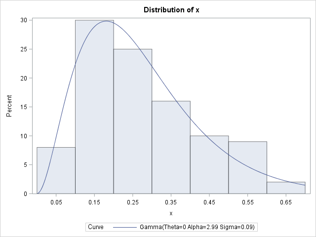
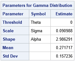
The parameter estimates are (2.99, 0.09), which are close to the parameter values that were used to generate the data. Notice that PROC UNIVARIATE does not provide standard errors or confidence intervals for these point estimates. However, you can get those statistics from PROC NLMIXED. PROC NLMIXED also supports the ESTIMATE statement, which can estimate the rate parameter:

/*Use PROC NLMIXED to fit the shape and scale parameters in a gamma model */
title "Fit Gamma Model, SCALE Parameter";
proc nlmixed data=Gamma;
   parms a 1 scale 1;             * initial value for parameter;
   bounds 0 < a scale;
   model x ~ gamma(a, scale);
   rate = 1/scale;
   estimate 'rate' rate;
   ods output ParameterEstimates=PE;
   ods select ParameterEstimates ConvergenceStatus AdditionalEstimates;
run;

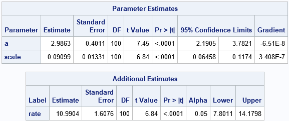
The parameter estimates are the same as from PROC UNIVARIATE. However, PROC NLMIXED also provides standard errors and confidence intervals for the parameters. More importantly, the ESTIMATE statement enables you to obtain an estimate of the rate parameter without needing to refit the model. The next section explains how the rate parameter is estimated.

New estimates and changing variables

You might wonder how the ESTIMATE statement computes the estimate for the rate parameter from the estimate of the scale parameter. The PROC NLMIXED documentation states that the procedure "computes approximate standard errors for the estimates by using the delta method (Billingsley 1986)." I have not studied the "delta method," but it seems to a way to approximate a nonlinear transformation by using the first two terms of its Taylor series, otherwise known as a linearization.

In the ESTIMATE statement, you supply a transformation, which is c = 1 / β for the gamma distribution. The derivative of that transformation is -1 / β². The estimate for β is 0.09. Plugging that estimate into the transformations give 1/0.09 as the point estimate for c and 1/0.09² as a linear multiplier for the size of the standard error. Geometrically, the linearized transformation scales the standard error for the scale parameter into the standard error for the rate parameter. The following SAS/IML statements read in the parameter estimates for β. It then uses the transformation to produce a point estimate for the rate parameter, c, and uses the linearization of the transformation to estimate standard errors and confidence intervals for c.

proc iml;
start Xform(p);
   return( 1 / p );          /* estimate rate from scale parameter */
finish;
start JacXform(p);
   return abs( -1 / p##2 );  /* Jacobian of transformation */
finish;
 
use PE where (Parameter='scale');
read all var {Estimate StandardError Lower Upper};
close;
 
xformEst = Xform(Estimate);
xformStdErr = StandardError * JacXform(Estimate);
CI = Lower || Upper;
xformCI = CI * JacXform(Estimate);
AdditionalParamEst = xformEst || xformStdErr || xformCI;
print AdditionalParamEst[c={"Est" "StdErr" "LowerCL" "UpperCL"} F=D8.4];
quit;

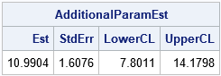
The estimates and other statistics are identical to those produced by the ESTIMATE statement in PROC NLMIXED. For a general discussion of changing variables in probability and statistics, see these Penn State course notes. For a discussion about two different parameterizations of the lognormal distribution, see the blog post "Geometry, sensitivity, and parameters of the lognormal distribution."

In case you are wondering, you obtain exactly the same parameter estimates and standard errors if you fit the rate parameter directly. That is, the following call to PROC NLMIXED produces the same parameter estimates for c.

/*Use PROC NLMIXED to fit gamma model using rate parameter */
title "Fit Gamma Model, RATE Parameter";
proc nlmixed data=Gamma;
   parms a 1 rate 1;             * initial value for parameter;
   bounds 0 < a rate;
   model x ~ gamma(a, 1/rate);
   ods select ParameterEstimates;
run;

For this example, fitting the scale parameter is neither more nor less difficult than fitting the rate parameter. If I were faced with a distribution that has two different parameterizations, one simple and one more complicated, I would try to fit the simple parameters to data and use this technique to estimate the more complicated parameters.