Today is my 500th blog post for The DO Loop. I decided to celebrate by doing what I always do: discuss a statistical problem and show how to solve it by writing a program in SAS.

Two ways to parameterize the lognormal distribution

I recently blogged about the relationship between the parameters in the lognormal family and the underlying normal family. This inspired me to look closer into how the mean and standard deviation of the normal distribution are related to the mean and standard deviation of the lognormal distribution.

Recall that if X ~ N(μ, σ) is normally distributed with parameters μ and σ, then Y = exp(X) is lognormally distributed with the same parameters. The mean of Y is m = exp(μ + σ²/2) and the variance is v = (exp(σ²) -1) exp(2μ + σ²). As usual, the standard deviation of Y is sqrt(v).

These formulas establish a one-to-one (and therefore invertible) relationship between the central moments (means and standard deviations) of the normal and lognormal distributions. If you have the lognormal parameters (m, sqrt(v)), you can compute the corresponding normal parameters, and vice versa. The formulas for μ and σ as functions of m and v are μ = ln(m² / φ) and σ = sqrt( ln(φ² / m²) ) where φ = sqrt(v + m²). You can think of these formulas as defining a function, F, that maps (m, sqrt(v)) values into (μ, σ) values.

What does this mapping tell us about the relationship between the central moments of the normal and lognormal distributions? What is the geometry of the transformation that maps one set of means and standard deviations to the other?

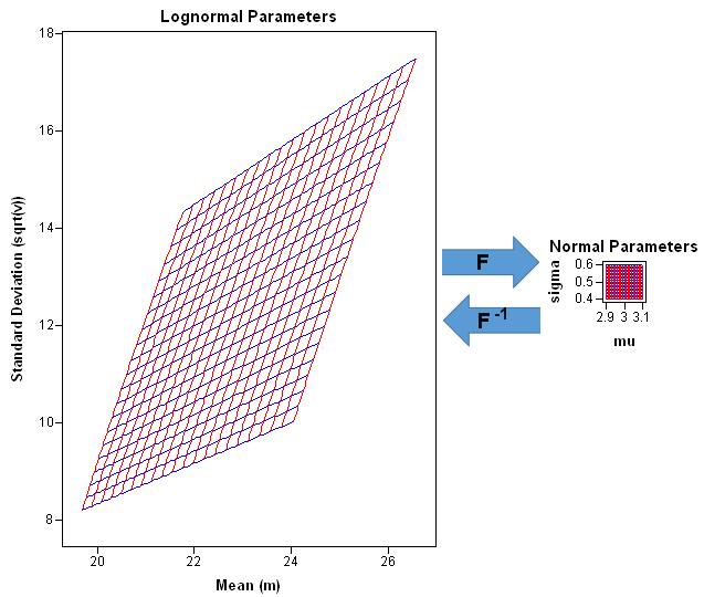
If F is the function that gives (μ, σ) as a function of (m, sqrt(v), you can visualize F by using the graphic to the left. (Click to enlarge.) The grid in the upper part of the picture represents a uniform mesh [1,30] x [1,30] in the domain of F. These are means and standard deviations for lognormal distributions. Vertical lines (m is constant) are drawn in red; horizontal lines (v is constant) are drawn in blue. The corresponding (μ, σ) values (the image of the grid under F) are shown in the bottom part of the picture. The bottom picture shows the mean and standard deviation of the corresponding normal distributions.

By looking at the scale of the graphs, you can see that the transformation is highly contractive on this domain. The function maps a huge rectangle (841 square units) into a little wing-shaped region whose area is about 11 square units. The contraction is especially strong when the lognormal parameters m and v are large. For example the entire right half of the grid in the domain of F (where m ≥ 15) is mapped into a tiny area near (μ,σ)=(3,0.5) in the range.

This fact is not too surprising because the inverse mapping (F^–1) is exponential, and therefore highly expansive. Nevertheless, it is illuminating to see the strength of the contraction. For example, the following graphic "zooms in" on an area of the domain that is centered near the point (m, sqrt(v)) = (22.5, 11.5), which is the approximate pre-image of (μ, σ) = (3, 0.5). The parallelogram in the domain of F is mapped to a tiny square that is centered near (μ, σ) = (3, 0.5). On this scale, the mapping is well-approximated by its linearization, which is the Jacobian matrix of first derivatives. The determinant of the Jacobian matrix at the point (m, sqrt(v) = (22.5, 11.5) is about 1/600, which means that the big parallelogram on the left has about 600 times the area of the tiny square on the right. (In the illustration, the square is not drawn to scale.)

Implications for data analysis

These pictures and computations tell us a lot about the relationship between the central moments of the normal and the lognormal distribution. The main result is that small changes in the parameters of the normal distribution cause large changes in the mean and standard deviation of the lognormal distribution. This leads to the following corollaries:

• Small variations in normal data can lead to big difference in the lognormal data. If you simulate a small sample of data from an N(3, 0.5) distribution, you will get a sample moments that vary slightly from the parameter values. For example, the sample mean might range between 2.9 and 3.1, and the sample standard deviation might range between 0.4 and 0.6. However, if you exponentiate the simulated values to form a lognormal distribution, the mean and standard deviation of the lognormal data will vary widely from sample to sample. In short, the mean and standard deviation of lognormal data are very sensitive to variation in the normal samples.
• For lognormal data with a large mean, the parameter estimates are not sensitive to variation in the data. Suppose you have a small data set with mean 22.5 and the standard deviation 11.5, and you think it lognormally distributed. If you use PROC UNIVARIATE to estimate the parameters for a lognormal fit, you will get estimates that are close to μ=3 and σ=0.5. Because of the small sample size, you might be worried that the parameter estimates aren't very good. But look at it this way: if you draw a different sample whose mean and standard deviation are several units away from those values, the parameter estimates will still be close to μ=3 and σ=0.5! Variations in the lognormal data are not very important when you estimate the parameters of the underlying normal data.

For simplicity, this discussion focused on parameter values near (μ, σ)=(3, 0.5), but you can use the same ideas and pictures to study other regions of parameter space. Moreover, the same ideas apply to other data transformations.

Computational details

The SAS/IML language is an excellent way to compute the quantities and to create the pictures in this article. In particular, I used the dynamically linked graphics in SAS/IML Studio to explore this problem because of the highly flexible graphics in IMLPlus. You can download the complete SAS/IML Studio program that I used to create the images.

The grids in the graphs were created by using the EXPANDGRID function that I discussed in the article how to generate a grid of points in SAS. It is easy to apply the transformation to the grid:

proc iml;
/* lognormal to normal transformation (m, sqrt(v)) --> (mu, sigma) */
start LN2N(p);
   m = p[,1]; v = p[,2]##2;
   phi = sqrt(v + m##2);
   mu = log(m##2 / phi);
   sigma = sqrt(log(phi##2/m##2));
   return( mu || sigma );
finish;
 
m = 1:30;                      /* horizontal grid points */
sqrtV = 1:30;                  /* vertical grid points */
grid = expandgrid(m, sqrtV);   /* make grid (SAS/IML 12.3) */
Fgrid = LN2N(grid);            /* compute image of grid */

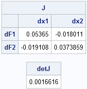
You can easily compute a numerical Jacobian matrix (the matrix of first derivatives) by using the NLPFDD function, which computes finite-difference derivatives. You can compute the determinant of the Jacobian matrix by using the DET function. The following statements compute the Jacobian matrix and determinant at the point (22.5, 11.5). The determinant is approximately 1/600.

/* NLPFDD wants a function that returns a column vector */
start LN2Ncol(x);  
   return( T(LN2N(x)) );
finish;
 
/* linearization of lognormal-->normal transformation */
x0 = {22.5 11.5};    /* approximate pre-image of (3, 0.5) */
call nlpfdd(f, J, JpJ, "LN2Ncol", x0, {2 . .});
detJ = det(J);       /* det(J) shows strong local contraction */
print J[c={"dx1" "dx2"} r={"dF1" "dF2"}], detJ;

This article—my 500th blog post—provides a good example of what I try to accomplish with my blog. The problem was inspired by a question from a SAS customer. I analyzed it by writing a SAS/IML program. The analysis requires applications of statistics, multivariate analysis, geometry, and matrix computations. I created some cool graphs. Thanks for reading.