A SAS customer asked how to simulate data from a three-parameter lognormal distribution as specified in the PROC UNIVARIATE documentation. In particular, he wanted to incorporate a threshold parameter into the simulation.

Simulating lognormal data is easy if you remember an important fact: if X is lognormally distributed, then Y=log(X) is normally distributed. The converse is also true: If Y is normally distributed, then X=exp(Y) is lognormally distributed. Consequently, to simulate lognormal data you can simulate Y from the normal distribution and exponentiate it to get X, which is lognormally distributed by definition. If you want, you can add a threshold parameter to ensure that all values are greater than the threshold.

Simulate a sample from a two-parameter lognormal distribution

To reiterate: if Y ~ N(μ, σ) is normally distributed with location parameter μ and scale parameter σ, then X = exp(Y) is lognormally distributed with log-location parameter μ and log-scale parameter σ. Different authors use different names for the μ and σ parameters. The PROC UNIVARIATE documentation uses the symbol ζ (zeta) instead of μ, and it calls ζ a scale parameter. Hence, I will use the symbol ζ, too. I have previously written about the relationship between the two lognormal parameters and the mean and variance of the lognormal distribution.

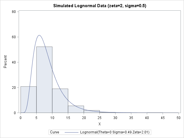
Regardless of what name and symbol you use, you can use the definition to simulate lognormal data. The following SAS DATA set simulates one sample of size 1000 from a lognormal distribution with parameters ζ=2 and σ=0.5. PROC UNIVARIATE then fits a two-parameter lognormal distribution to the simulated data. The maximum likelihood estimates for the sample are 2.01 and 0.49, so the estimates from the simulated data are very close to the parameter values:

ods graphics/reset;
%let N = 1000;          /* sample size */
data LN1;
call streaminit(98765);
sigma = 0.5;      /* shape or log-scale parameter    */
zeta = 2;         /* scale or log-location parameter */
do i = 1 to &N;
   Y = rand("Normal", zeta, sigma);  /* Y ~ N(zeta, sigma)    */
   X = exp(Y);                       /* X ~ LogN(zeta, sigma) */
   output;
end;
keep X;
run;
 
proc univariate data=LN1;      /* visualize simulated data and check fit */
   histogram X / lognormal endpoints=(0 to 50 by 5)
                 odstitle="Simulated Lognormal Data (zeta=2, sigma=0.5)";
run;

Simulate many samples from a three-parameter lognormal distribution

You can modify the previous program to simulate from a lognormal distribution that has a threshold parameter. You simply add the threshold value to the exp(Y) value, like this: X = theta + exp(Y). Because exp(Y) is always positive, X is always greater than theta, which is the threshold value.

In Monte Carlo simulation studies, you often want to investigate the sampling distribution of the model parameter estimates. That is, you want to generate many samples from the same model and see how the estimates differ across the random samples. The following DATA step simulates 500 random samples from the three-parameter lognormal distribution with threshold value 10. You can analyze all the samples with one call to PROC UNIVARIATE that uses the BY statement to identify each sample. This is the efficient way to perform Monte Carlo simulation studies in SAS.

%let N = 100;          /* sample size */
%let NumSamples = 500; /* number of samples */
%let Threshold = 10;   
data LN;               /* generate many random samples */
call streaminit(98765);
sigma = 0.5;      /* shape or log-scale parameter    */
zeta = 2;         /* scale or log-location parameter */
do SampleID = 1 to &NumSamples;
   do i = 1 to &N;
      Y = rand("Normal", zeta, sigma);
      X = &Threshold + exp(Y);
      output;
   end;
end;
keep SampleID X;
run;
 
ods exclude all;                 /* do not produce tables during analyses */
proc univariate data=LN;
   by SampleID;                  /* analyze the many random samples */
   histogram x / lognormal(theta=&Threshold); /* 2-param estimation */
   ods output parameterestimates=PE;
run;
ods exclude none;
 
data Estimates;                 /* convert from long to wide for plotting */
keep SampleID Zeta Sigma;
merge PE(where=(Parameter="Scale") rename=(Estimate=Zeta))
      PE(where=(Parameter="Shape") rename=(Estimate=Sigma));
by sampleID;
label Zeta="zeta: Estimates of Scale (log-location)"
      Sigma="sigma: Estimate of Shape (log-scale)";
run;
 
title "Approximate Sampling Distribution of Lognormal Estimates";
title2 "Estimates from &NumSamples Random Samples (N=&N)";
proc sgplot data=Estimates;
   scatter x=Zeta y=Sigma;
   refline 2 / axis=x;
   refline 0.5 / axis=y;
run;

The distribution of the 500 estimates appears to be centered on (ζ, σ) = (2, 0.5), which are the parameter values that were used to simulate the data. You can use the usual techniques in Monte Carlo simulation to estimate the standard deviation of the estimates.

A few closing remarks:

• The RAND function does not support location and scale parameters for the lognormal distribution in SAS in 9.4m4. However, the RANDGEN function in SAS/IML does support two-parameter lognormal parameters. The RAND function will support lognormal parameters in 9.4m5.
• In this study, the estimates are all two-parameter estimates, which assumes that you know the threshold value in the population. If not, you can use THETA=EST on the HISTOGRAM statement to obtain three-parameter lognormal estimates.
• Because you need to exponentiate the Y variable, random values of Y must be less than the value of CONSTANT('logbig'), which is about 709. To avoid numerical overflows, make sure that ζ + 4*σ is safely less than 709.
• This sort of univariate simulation is discussed in detail in Chapter 7 of the book Simulating Data with SAS, along with a general discussion about how to simulate from location-scale families even for distributions for which the RAND function does not support location or scale parameters.