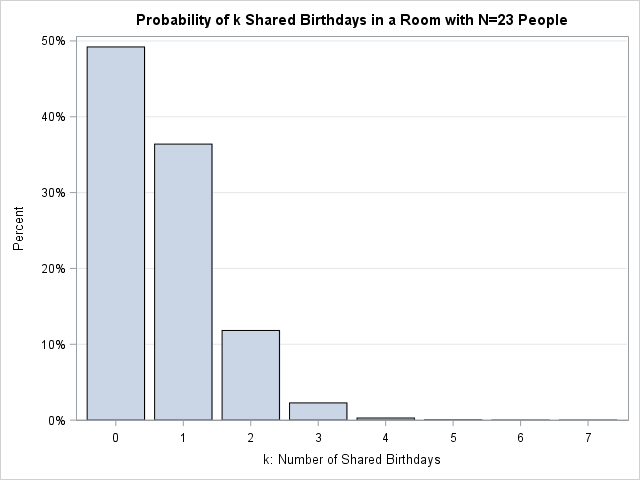
If N random people are in a room, the classical birthday problem provides the probability that at least two people share a birthday. The birthday problem does not consider how many birthdays are in common. However, a generalization (sometimes called the Multiple-Birthday Problem) examines the distribution of the number of shared birthdays. Specifically, among N people, what is the probability that exactly k birthdays are shared (k = 1, 2, 3, ..., floor(N/2))? The bar chart at the right shows the distribution for N=23. The heights of the bars indicate the probability of 0 shared birthdays, 1 shared birthday, and so on.

This article uses simulation in SAS to examine the multiple-birthday problem. If you are interested in a theoretical treatment, see Fisher, Funk, and Sams (2013, p. 5-14).

The probability of multiple shared birthdays for N=23

You can explore the classical birthday problem by using probability theory or you can estimate the probabilities by using Monte Carlo simulation. The simulation in this article assumes 365 equally distributed birthdays, but see my previous article to extend the simulation to include leap days or a nonuniform distribution of birthdays.

The simulation-based approach enables you to investigate the multiple birthday problem. To begin, consider a room that contains N=23 people. The following SAS/IML statements are taken from my previous article. The Monte Carlo simulation generates one million rooms of size 23 and estimates the proportion of rooms in which the number of shared birthdays is 0, 1, 2, and so forth.

proc iml;
/* Function that simulates B rooms, each with N people, and counts the number of shared 
   (matching) birthdays in each room. The return value is a row vector that has B counts. */
start BirthdaySim(N, B);                 
   bday = Sample(1:365, B||N);             /* each column is a room */
   match = N - countunique(bday, "col");   /* number of unique birthdays in each col */
   return ( match );
finish;
 
call randseed(12345);                      /* set seed for random number stream */
NumPeople = 23;
NumRooms = 1e6;
match = BirthdaySim(NumPeople, NumRooms);  /* 1e6 counts */
 
call tabulate(k, freq, match);  /* summarize: k=number of shared birthdays, freq=counts */ 
prob = freq / NumRooms;         /* proportion of rooms that have 0, 1, 2,... shared birthdays */
print prob[F=BEST6. C=(char(k,2)) L="Estimate of Probability (N=23)"];

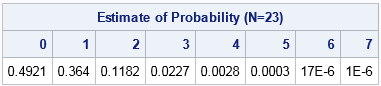
The output summarizes the results. In less than half the rooms, no person shared a birthday with anyone else. In about 36% of the rooms, one birthday is shared by two or more people. In about 12% of the room, there were two birthdays that were shared by four or more people. About 2% of the rooms had three birthdays shared among six or more individuals, and so forth. In theory, there is a small probability of a room in which 8, 9, 10, or 11 birthdays are shared, but the probability of these events is very small. The probability estimates are plotted in the bar chart at the top of this article.

There is a second way to represent this probability distribution: you can create a stacked bar chart that shows the cumulative probability of k or fewer shared birthdays for k=1, 2, 3,.... You can see that the probability of 0 matching birthdays is less than 50%, the probability of 1 or fewer matches is 87%, the probability of 2 or fewer matches is 97%, and so forth. The probability for 5, 6, or 7 matches is not easily determined from either chart.

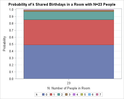
Mathematically speaking, the information in the stacked bar chart is equivalent to the information in the regular bar chart. The regular bar chart shows the PMF (probability mass function) for the distribution whereas the stacked chart shows the CDF (cumulative distribution function).

The probability of shared birthdays among N people

The previous section showed the distribution of shared birthdays for N=23. You can download the SAS program that simulates the multiple birthday problem for rooms that contain N=2, 3, ..., and 60 people. For each simulation, the program computes estimates for the probabilities of k matching birthdays, where k ranges from 0 to 30.

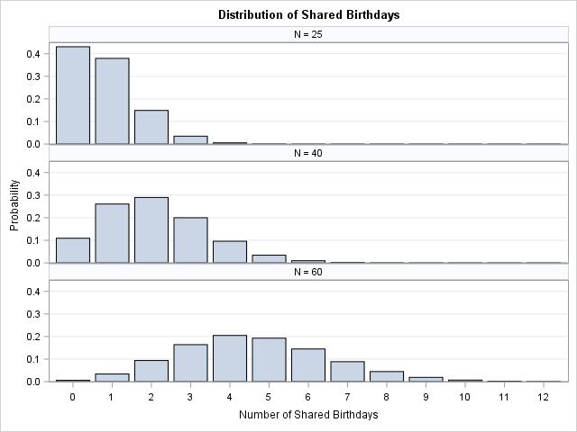
There are a few ways to visualize those 59 distributions. One way is to plot 59 bar charts, either in a panel or by using an animation. A panel of three bar charts is shown to the right for rooms of size N=25, 40, and 60. You can see that the bar chart for N=25 is similar to the one shown earlier. For N=40, most rooms have between one and three shared birthdays. For rooms with N=60 people, most rooms have between three and six shared birthdays. The horizontal graphs are truncated at k=12, even though a few simulations generated rooms that contain more than 12 matches.

Obviously plotting all 59 bar charts would require a lot of space. A different way to visualize these 59 distributions is to place 59 stacked bar charts side by side. This visualization is more compact. In fact, instead of 59 stacked bar charts, you might want to create a stacked band plot, which is what I show below.

The following stacked band chart is an attempt to visualize the distribution of shared birthdays for ALL room sizes N=2, 3, ..., 60. (Click to enlarge.)

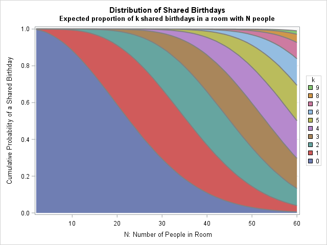
How do you interpret this graph? A room that contains N=23 people corresponds to drawing a vertical line at N=23. That vertical line intersects the red, green, and brown bands near 0.5, 0.87, and 0.97. Therefore, these are the probabilities that a room with 23 people contains 0 shared birthdays, 1 or fewer shared birthdays, and 2 or fewer shared birthdays. The vertical heights of the bands qualitatively indicate the individual probabilities.

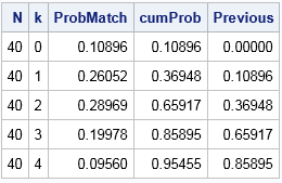
Next consider a room that contains N=40 people. A vertical line at N=40 intersects the colored bands at 0.11, 0.37, 0.66, 0.86, and 0.95. These are the cumulative probabilities P(k ≤ 0), P(k ≤ 1), P(k ≤ 2), and so forth. If you need the exact values, you can use PROC PRINT to display the actual probability estimates. For example:

proc print data=BDayProb noobs;
   where N=40 and k < 5;
run;

Summary

In summary, this article examines the multiple-birthday problem, which is a generalization of the classical birthday problem. If a room contains N random people, the multiple-birthday problem examines the probability that k birthdays are shared by two or more people for k = 0, 1, 2, ..., floor(N/2). This article shows how to use Monte Carlo simulation in SAS to estimate the probabilities. You can visualize the results by using a panel of bar charts or by using a stacked band plot to visualize the cumulative distribution. You can download the SAS program that simulates the multiple birthday problem, estimates the probabilities, and visualizes the results.

What do you think? Do you like the stacked band plot that summarizes the results in one graph, or do you prefer a series of traditional bar charts? Leave a comment.