This article simulates the birthday-matching problem in SAS. The birthday-matching problem (also called the birthday problem or birthday paradox) answers the following question: "if there are N people in a room, what is the probability that at least two people share a birthday?" The birthday problem is famous because the probability of duplicate birthdays is much higher than most people would guess: Among 23 people, the probability of a shared birthday is more than 50%.

If you assume a uniform distribution of birthdays, the birthday-matching problem can be solved exactly. In reality birthdays are not uniformly distributed, but as I show in Statistical Programming with SAS/IML Software (Wicklin 2010), you can use a Monte Carlo simulation to estimate the probability of a matching birthday.

This article uses ideas from Wicklin (2010) to simulate the birthday problem in the SAS/IML language. The simulation is simplest to understand if you assume uniformly distributed birthdays (p. 335–337), but it is only slightly harder to run a simulation that uses an empirical distribution of birthdays (p. 344–346). For both cases, the simulation requires only a few lines of code.

Monte Carlo estimates of the probabilities in the birthday problem

The birthday-matching problem readily lends itself to Monte Carlo simulation. Represent the birthdays by the integers {1, 2, ..., 365} and do the following:

1. Choose a random sample of size N (with replacement) from the set of birthdays. That sample represents a "room" of N people.
2. Determine whether any of the birthdays in the room match. There are N(N-1)/2 pairs of birthdays to check.
3. Repeat this process for thousands of rooms and compute the proportion of rooms that contain a match. This is a Monte Carlo estimate of the probability of a shared birthday.
4. If desired, simulate rooms of various sizes, such as N=2, 3, 4,..., 60, and plot the results.

How to simulate the birthday problem in SAS

Before running the full simulation, let's examine a small-scale simulation that simulates only 10 rooms, each containing a random sample of N = 23 people:

proc iml;
call randseed(12345);                 /* set seed for random number stream */
N = 23;                               /* number of people in room */
NumRooms = 10;                        /* number of simulated rooms */
bday = Sample(1:365, NumRooms||N);    /* simulate: each column is a room that contains N birthdays */
*print bday;                          /* optional: print the 23 x 10 matrix of birthdays */
match = N - countunique(bday, "col"); /* number of unique birthdays in each col */
print match[label="Num Matches (N=23)" c=("Rm1":"Rm10")];
 
/* estimate the probability of a match, based on 10 simulations */
probMatch = (match > 0)[:];          /* mean = proportion of matches */
print probMatch;

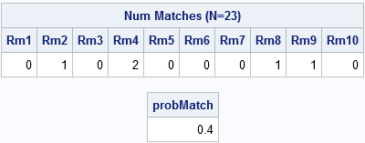
The output shows the number of matches in 10 rooms, each with 23 people. The first room did not contain any people with matching birthdays, nor did rooms 3, 5, 6, 7, and 10. The second room contained one matching birthday, as did rooms 8 and 9. The fourth room contains two shared birthdays. In this small simulation, 4/10 of the rooms contain a shared birthday, so the Monte Carlo estimate of the probability is 0.4. You can compute the estimate by forming the binary indicator variable (match > 0) and computing the mean. (Recall that the mean of a binary vector is the proportion of 1s.)

Notice that the simulation requires only three SAS/IML vectorized statements. The SAMPLE function produces a matrix that has N rows. Each column of the matrix represents the birthdays of N people in a room. The COUNTUNIQUE function returns a row vector that contains the number of unique birthdays in each column. If you subtract that number from N, you obtain the number of shared birthdays. Finally, the estimate is obtained by computing the mean of an indicator variable.

Simulate the birthday problem in SAS

For convenience, the following SAS/IML statements define a function that simulates B rooms, each containing a random sample of N birthdays. The function returns a row vector of size B that contains the number of matching birthdays in each room. The program calls the function in a loop and graphs the results.

start BirthdaySim(N, B);
   bday = Sample(1:365, B||N);           /* each column is a room */
   match = N - countunique(bday, "col"); /* number of unique birthdays in each col */
   return ( match );
finish;
 
maxN = 60;                    /* consider rooms with 2, 3, ..., maxN people */
NumPeople = 2:maxN;
probMatch = j(MaxN, 1, 0);    /* allocate vector for results */
NumRooms = 10000;             /* number of simulated rooms */
 
do N = 1 to ncol(NumPeople);
   match =  BirthdaySim(NumPeople[N], NumRooms);
   probMatch[N] = (match > 0)[:];
end;
 
title "The Birthday Matching Problem";
call series(NumPeople, probMatch) grid={x y} 
     label={"Number of People in Room" "Probability of a Shared Birthday"};

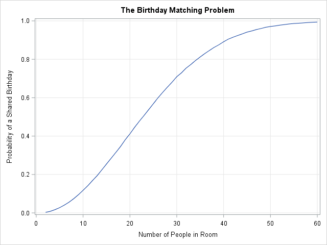
The graph is shown at the top of this article. It shows the estimated probability of one or more matching birthdays in a room of size N for N=2, 3, ..., 60. The estimates are based on 10,000 Monte Carlo iterations. (Why did I use 10,000 rooms? See the Appendix.) As mentioned earlier, the probability exceeds 50% when a room contains 23 people. For 30 people, the probability of a match is 71%. If you put 50 people in a room, the chances that two people in the room share a birthday is about 97%.

Allow leap days and a nonuniform distribution of birthdays

The curious reader might wonder how this analysis changes if you account for people born on leap day (February 29th). The answer is that the probabilities of a match decrease very slightly because there are more birthdays, and you can calculate the probability analytically. If you are interested in running a simulation that accounts for leap day, use the following SAS/IML function:

start BirthdaySim(N, B);
   /* A four-year period has 3*365 + 366 = 1461 days. Assuming uniformly distributed 
      birthdays, the probability vector for randomly choosing a birthday is as follows: */
   p = j(366, 1, 4/1461);      /* most birthdays occur 4 times in 4 years */
   p[31+29] = 1/1461;          /* leap day occurs once in 4 years */
   /* sample with replacement using this probability of selection */
   bday = Sample(1:366, B||N, "replace", p);           /* each column is a room */
   match = N - countunique(bday, "col"); /* number of unique birthdays in each col */
   return ( match );
finish;

If you run the simulation, you will find that the estimated probability of sharing a birthday among N people does not change much if you include leap-day birthdays. The difference between the estimated probabilities is about 0.003 on average, which is much less than the standard error of the estimates. In practice, you can exclude February 29 without changing the conclusion that shared birthdays are expected to occur.

In a similar way, you can set the probability vector to be the empirical distribution of birthdays in the population. Wicklin (2010, p. 346) reports that the simulation-based estimates are slightly higher than the exact results that you obtain from assuming a uniform distribution. This agrees with theory: A. G. Munford (TAS, 1977) showed that any nonuniform distribution increases the likelihood of a matching birthday. In other words, in the real world, the probability of a shared birthday is slightly higher than in the idealized mathematical world.

Appendix: How many Monte Carlo simulations are necessary?

Why did I use 10,000 Monte Carlo simulations? Notice that the Monte Carlo estimate in this problem is an estimate of a proportion of a binary variable, which means that you can estimate the standard error. If p̂ is the estimate, then a 95% confidence interval has radius 1.96 sqrt(p̂(1-p̂)/B), where B is the number of Monte Carlo simulations (that is, the number of "rooms"). This quantity is largest when p̂ = 1/2, so if you want, say, two digits of accuracy you can choose a value of B which is large enough so that 1.96 sqrt(0.5(1-0.5)/B) ≤ 0.01. Solving the equation for B give B ≥ 10000. If you choose that many Monte Carlo iterations, then the conservative 95% confidence interval has a half-width no greater than 0.01.

This simple calculation shows that if you use B=10,000 for the number of simulated "room," you can expect the Monte Carlo estimates to be within 0.01 of the true probability 95% of the time. The standard error is largest where the curve is steepest (near N=23). You could add error bars to the graph, but the errors would be too small to see.