To a statistician, the DIF function (which was introduced in SAS/IML 9.22) is useful for time series analysis. To a numerical analyst and a statistical programmer, the function has many other uses, including computing finite differences.

The DIF function computes the difference between the original vector and a shifted version of that vector. In terms of the LAG function, DIF(x,k) = x - LAG(x,k) for any value of the lag parameter, k. I blogged about the usefulness of the LAG function earlier this week.

Using the DIF function to compute forward and backward differences

For a function that is given by a formula, you can use the NLPFDD subroutine to compute finite difference derivatives. However, sometimes a function is known only at a finite set of points. In that case, you have a choice: you can either model the function by using regression techniques or you can assume that the function is piecewise linear.

Some curves really are piecewise linear. For example, an ROC curve is piecewise linear, and you can compute the exact derivatives by using a forward or backward difference scheme. You can also compute an exact area under the piecewise linear function by using the trapezoidal rule of integration.

The DIF function makes it easy to compute lagged differences (finite differences) in a sequence of values. As an example, the derivative of a function can be approximated by the backward difference formula: f'(x) ≈ (f(x)-f(x-h))/h for small values of h. If you know the values of f at a discrete set of points x₁ < x₂ < ... < x_n, then you can use the DIF function to evaluate the backward difference because the expression f(x_i-h) is the lagged term f(x_i-1). For example, the following SAS/IML program computes a sequence of evenly spaced x values and evaluates the sine function at these points. The points of the backDiff vector approximate the derivative of the sine at each value of x:

proc iml;
h = 0.1;
x = T( do(0, 6.28, h) );
y = sin(x);
backDiff =  dif(y, 1) / h;     /* f'(x) ~ (f(x)-f(x-h))/h */

When the DIF function is called with a single argument, a lag of 1 is assumed, so you can also write backDiff = dif(y)/h.

We know from calculus that the exact derivative of the sine function is the cosine. The following function computes the exact derivative at each value of x and compares it with the finite difference approximation:

deriv = cos(x);
maxBDiff = max(abs(deriv-backDiff)); /* find maximum difference */
print maxBDiff;

The following plot shows the exact derivative and the backward difference approximation at each point of x:

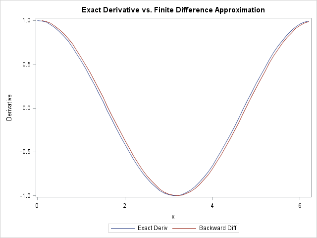
The finite difference approximations are in close agreement with the exact values. You can also plot the forward difference approximation, which is similar. The forward difference requires using a shift value of -1. When you work through the formula, you find that forwardDiff = -dif(y, -1) / h.

Finite differences for irregularly spaced data

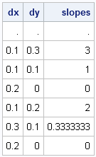
The DIF function also "works" on irregularly spaced data. For data that are not evenly spaced, the h parameter, which is the difference between adjacent x values, is no longer constant. You can use the DIF function to compute the distance between x values, and then compute the slopes as shown in the following statements:

/* irregular spacing and no formula */
x = {0.0, 0.1, 0.2, 0.4, 0.5, 0.8, 1.0};
y = {0.3, 0.6, 0.7, 0.7, 0.9, 1.0, 1.0};
dx = dif(x);  /* difference for adjacent x values (lag=1) */
dy = dif(y);  /* difference for adjacent y values (lag=1) */
slopes = dy/dx;
print dx dy slopes;

You can also use the DIF and LAG function to implement integration schemes. For example, in my article on the trapezoidal rule of integration, I could have implemented the trapezoidal rule by using LAG and DIF instead of using indexes to form the lag of the data vectors manually.