There are many techniques for generating random variates from a specified probability distribution such as the normal, exponential, or gamma distribution. However, one technique stands out because of its generality and simplicity: the inverse CDF sampling technique. If you know the cumulative distribution function (CDF) of a probability distribution, then you can always generate a random sample from that distribution. The inverse CDF technique for generating a random sample uses the fact that a continuous CDF, F, is a one-to-one mapping of the domain of the CDF into the interval (0,1). Therefore, if U is a uniform random variable on (0,1), then X = F–1(U) has the distribution F.
This article is taken from Chapter 7 of my book Simulating Data with SAS.
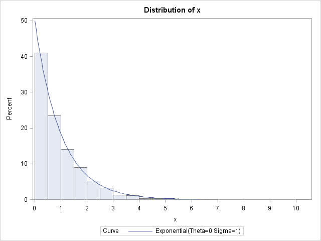
To illustrate the inverse CDF sampling technique (also called the inverse transformation algorithm), consider sampling from a standard exponential distribution. The exponential distribution has probability density f(x) = e–x, x ≥ 0, and therefore the cumulative distribution is the integral of the density: F(x) = 1 – e–x. This function can be explicitly inverted by solving for x in the equation F(x) = u. The inverse CDF is x = –log(1–u).
The following DATA step generates random values from the exponential distribution by generating random uniform values from U(0,1) and applying the inverse CDF of the exponential distribution. (Of course, the simpler way is to use x = RAND("Expo")!) The UNIVARIATE procedure is used to check that the data follow an exponential distribution. This example comes from Ross (2006, Fourth Edition).
/* Example of using the inverse CDF algorithm to generate variates from the exponential distribution */ data Exp(keep=x); call streaminit(1234); do i = 1 to 1000; /* sample size = 1000 */ u = rand("Uniform"); /* statistically equivalent to */ x = -log(1-u); /* x = rand("Expo"); */ output; end; run; ods select histogram; proc univariate data=Exp; histogram x / exponential(sigma=1) endpoints=0 to 10 by 0.5; run; |
In SAS, the QUANTILE function implements the inverse CDF function. That means that you can use the QUANTILE function to generate random variates. For example, the following statement is an equivalent way to use the inverse CDF method to generate exponential random variates:
u = rand("Uniform"); x = quantile("Expo", u); |
Although powerful, this inverse CDF method can be computationally expensive unless you have a formula for the inverse CDF. In SAS the QUANTILE function implements the inverse CDF function, but for many distributions it has to numerically solve for the root of the equation F(x) = u.
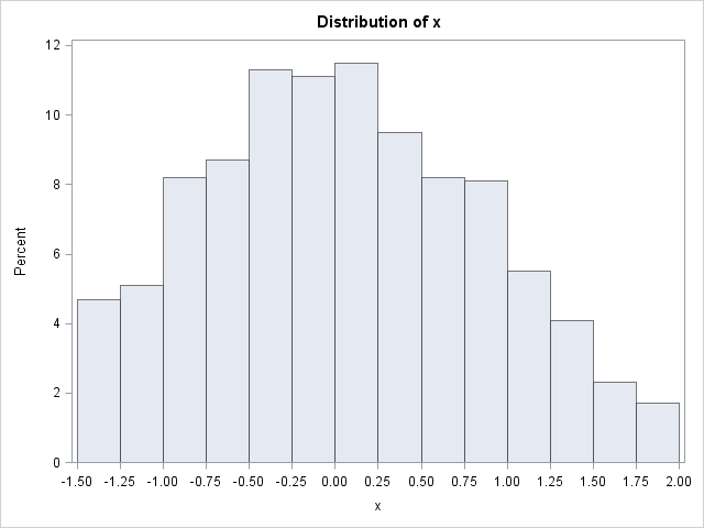
The inverse CDF technique is particularly useful when you want to generate data from a truncated distribution. For a distribution F, if you generate uniform random variates on the interval [F(a), F(b)] and then apply the inverse CDF, the resulting values follow the F distribution truncated to [a, b]. For example, to simulate a variate from the truncated normal distribution on [–1.5, 2], use the following statements:
/* Inverse CDF algorithm for truncated normal distribution on [a,b] */ data TruncNormal(keep=x); Fa = cdf("Normal", -1.5); /* for a = -1.5 */ Fb = cdf("Normal", 2.0); /* for b = 2.0 */ call streaminit(1234); do i = 1 to 1000; /* sample size = 1000 */ v = Fa + (Fb-Fa)*rand("Uniform"); /* V ~ U(F(a), F(b)) */ x = quantile("Normal", v); /* truncated normal on [a,b] */ output; end; run; ods select histogram; proc univariate data=TruncNormal; histogram x / endpoints=-1.5 to 2.0 by 0.25; run; |
WANT MORE GREAT INSIGHTS MONTHLY? | SUBSCRIBE TO THE SAS TECH REPORT

26 Comments
Numerical Solution for the inverse transform method
This question is Not Answered.(Mark as assumed answered)
Dede Atem
Novice
Dede Atem Dec 30, 2013 8:53 AM
Consider the following .
C= know value
U is Uniform (0,1)
F(x)=1-S(x) is well known
a=known value
k=known value
ht-= is known.
The only unknown is X.
I wish to write a SAS code that find X such that the right hand sight is equal the left hand side numerically.
I can not make X the subject but can find a numerical solution.
C*U=F(x) *exp(-(k-a*X)**2 - (k - a**2 * X) exp(-(k -a*X)**2/2t)*F(x)- ht
16 Views Tags: none (add)
This is a root-finding problem. For each given value of U, numerically find the value of X such that
C*U - RHS(X) = 0
You can use the FROOT function in SAS/IML, or use a bisection method (search my blog for 'bisection').
how to calaculate icdf for nakagami distribution
As stated on Wikipedia, a Nakagami random variable is just the square root of a gamma random variable. The CDF is given explicitly in terms of the incomplete gamma function, so use the CDF('GAMMA',...) function in SAS for the CDF and the QUANTILE('GAMMA',...) for the icdf.
Hi Rick,
How can one use the inverse cdf method to generate random samples from an unknown probability distribution, whose cdf is not invertible? For example, I have valid one dimensional density which has the following cdf:
F(x)=(exp(theta*(1-exp(-(alpha*x)^(beta))))-1)*[1+ lambda-lambda*[(exp(theta*(1-exp(-(alpha*x)^(beta))))-1)]/((exp(theta)-1))].
Let me know how to tackle this one.
Thanks,
Indranik
A continuous CDF is always invertible, but sometimes there is no formula for the inverse function. As I say in the second-to-last paragraph, in that case you need to use a root-finding method. For each u ~ U(0,1), solve the equation u = F(x) for x. In SAS/IML, you can use the FROOT function to find roots.
Pingback: The Lambert W function in SAS - The DO Loop
Hi Rick, does SAS have something like the matlab function EMPRAND (https://www.mathworks.com/matlabcentral/fileexchange/7976-random-number-from-empirical-distribution?requestedDomain=www.mathworks.com)
this function can generate a random number, given an empirical CDF.
Thank!
Adam
Great question. It might not seem obvious, but as I point out in my book, a drawing random sample from the empirical CDF is accomplished through basic bootstrap (re)sampling. If you want the ability to generate random values that are not in the original sample, the technique becomes the smooth bootstrap. If you choose to use a piecewise linear estimate to the ECDF, you get the technique in the article "Approximating a distribution from published quantiles."
hi Rick, thanks for sharing.
Suppose I have propensity score for a bunch of patients, and i have the ECDF of the PScore. if I want to draw a group of patients with similar ECDF from control patients, how can i sample based on a continuous CDF?
Given the complexity of this question, I suggest you ask it at the SAS Support Community for Statistical Procedures.
please sir what is the quantile form of hypertabastic model
I don't know. Most distributions do not have an explicit inverse in terms of elementary functions.
Hi Dr Rick,
How to obtain the inverse cdf of generalised gaussian distribution?
https://en.wikipedia.org/wiki/Generalized_normal_distribution
The generalized normal is defined in terms of the incomplete gamma function, which is a scaled version of the gamma distribution. Therefore you can invert the generalized normal CDF by using the quantile function of the gamma distribution. I suggest you do the inversion twice: once for y greater than mu and again for y less than mu. That eliminates the absolute value and the SIGN function.
hi rick, how would one use the integral transform method, without numerical inversion of for example the Gamma distribution?
Sorry, but I do not understand your question. I suggest you post your question at the SAS Support Communities. If the information in this article is relevant, link to it in your question. In your question, you should explain what you mean by "the integral transform method, without numerical inversion."
Suppose you are tasked with simulating a process where the inter-arrival times are not exponentially distributed, but Gamma(2, λ) under the fixed-count scheme, say 25 events, subject to the constraint that you must use the integral transform method of the Gamma distribution.
Im working using R.
The code below is what i used for an exponential distribution:
1 R> n = 25
2 R> lambda = 10
3 R> u = runif(n,0,1)
4 R> t = -1/lambda*log(1-u)
How would you modify it for a gamma distribution simulation.
Thanks
If you want help with R code, post your question to an R discussion list.
Pingback: Tips to simulate binary and categorical variables - The DO Loop
Pingback: The probability integral transform - The DO Loop
Pingback: Construct an envelope function for the acceptance-rejection method - The DO Loop
Pingback: The linear distribution on an interval - The DO Loop
Pingback: Latin hypercube sampling in SAS - The DO Loop
Pingback: The Lambert W function in SAS - The DO Loop
Pingback: Implement the Burr distribution in SAS - The DO Loop