Latin hypercube sampling in SAS

While researching the topic of Latin hypercube sampling (LHS), I read an article by Emily Gao (2019) that shows how to use PROC IML in SAS to perform the algorithm. It is possible to simplify Gao's implementation of Latin hypercube sampling in SAS while also making the computation more efficient. I do this by using two helper functions and a main function:

Helper function 1: Given an interval, [a,b], and a positive integer, k, divide the interval into k equal-width subintervals. Return a vector of values such the i_th value is positioned uniformly at random within the i_th subinterval. This can be done in a vectorized way without writing any loops.
Helper function 2: Given a matrix, M, randomly permute the rows of M. You can use the SAMPLE function in SAS IML to vectorize this step and avoid writing a loop.
Main function: Given a set of d intervals and positive integer, k, apply the previous functions to obtain k random positions within each of the d intervals.

The third step results in a random Latin hypercube sample. This sample is useful for exploring high-dimensional parameter spaces, such as for tuning hyperparameters and other machine learning purposes.

What is a Latin square?

A Latin square is familiar to researchers who have studied experimental design. The square is a k x k array that is filled with k symbols (usually Latin letters A, B, C,...) that each occur exactly once in each row and once in each column. In SAS, you can use the PLAN procedure to generate Latin square designs. For example, the following call to PROC PLAN is a small modification of a documentation example that constructs a 4 x 4 Latin square with the symbols A, B, C, and D:

proc plan seed=45;
   factors Row=4 ordered Col=4 ordered / noprint;
   treatments Values=4 cyclic;
   output out=LatinSquare Values cvals=('A' 'B' 'C' 'D') random
          Row nvals=(1 to 4) random
          Col nvals=(1 TO 4) random;
quit;

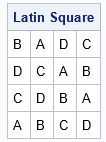
A Latin square uses two factors and results in a square array. You can add additional factors, which results in a Latin cube (three factors) or a Latin hypercube (more than 3 factors).

If you look ONLY at the positions of one of the symbols, you get a Latin hypercube sample. In the example, which has four symbols, there are four samples, one for each letter:

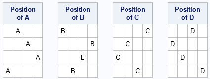
These are four of the 24 possible Latin square samples for a 4 x 4 Latin square. You can change the SEED= option on the PROC PLAN statement to see other possible random Latin squares.

Traditionally, a Latin square is used for discrete, categorical factors. However, if you have a continuous factor, you can discretize it into bins of equal size. For example, a continuous factor that can have values in [0,4] can be binned into subintervals [0,1), [1,2), [2,3), and [3,4]. You can think of each interval as being analogous to a level of a categorical variable.

Gao (2019) shows how to generate a random point in each subinterval for each factor while preserving the defining feature of a Latin square, which is that no row or column contains more than one observation. The next sections demonstrate an alternative way to generate the subintervals and random points within the subintervals.

Helper function: Generate random positions within subintervals

This section introduces a helper function, UnifSampleSubIntervals, which subdivides a interval into k subintervals, then returns a random point within each subinterval.

Fact: Given any interval [L,R], if u ~ U(0,1) is a random variate from the uniform distribution on (0,1), then the value t = L + (R-L)*u is a random position within the interval.

You can use this fact to generate positions uniformly at random within k evenly spaced subintervals of an interval. For an interval [a,b], let h = (b-a)/k be the width of the k subintervals. Then the left-hand endpoints of the intervals look like L[i]= a + h*i for i=1,2,...,k-1. Consequently, if u is a random uniform variate, the position t[i]= L[i]+ h*u is random within the i_th subinterval. The following call to PROC IML defines a function that generates random points in k subintervals:

proc iml;
/* specify an interval [a,b] and a number of subintervals.
   Divide [a,b] into <em>k</em> subintervals and return a point uniformly at random within each subinterval.
*/
start UnifSampleSubIntervals(interval, k);
   a = interval[1];
   b = interval[2];
   h = (b-a)/k;
   L = colvec( do(a, b-h/2, h) ); /* left-hand endpoints of k subintervals */
   u = randfun(k, "Uniform");     /* vector of random proportions */
   eta = L + u*h;   /* eta[i] is randomly located in the i_th subinterval */
   return( eta );
finish;
 
call randseed(1234);
t = UnifSampleSubIntervals({0 1}, 4);  /* subdivide [0,1] into 4 subintervals */

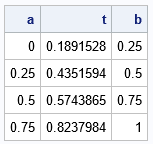
The output shows the four evenly spaced subintervals of [0,1] along with a random point (t) in each subinterval. The random point can be anywhere in the interval.

Helper function: Randomly permute rows of a matrix

In addition to random points within subintervals, Latin hypercube sampling requires randomly permuting the intervals. You can use the SAMPLE function to randomly permute the rows of a matrix. Suppose a vector or matrix has k rows. The SAMPLE function can return a random sample without replacement of the set {1,2,...,k}. This random sample represents a random permutation. Consequently, if M is a matrix and p is a random permutation, then M[p,] is the IML notation for randomly permuting the rows. This is implemented by using the following function:

/* helper function: Use the SAMPLE function to permute the rows of a matrix */
start PermuteRows(M);
   k = nrow(M);
   p = sample(1:k, k, "WOR");  /* random permutation of 1:k */
   return( M[p, ] );
finish;

Step 3: Implement Latin hypercube sampling

Gao (2019) was interested in a specific type of Latin hypercube sampling. She wanted to be able to specify d intervals and a positive integer, k, and obtain a k x d matrix where the columns represent random points in k subintervals within each of the intervals. The rows represent k points in d-dimensional space. These rows can be used for a tuning d hyperparameters in a machine learning models, among other uses. See Gao (2019) for a discussion of how LHS is useful in machine learning.

With the two helper functions, the implementation of LHS is short and efficient:

/* LHS: Latin hypercube sampling. Generate random location within k subintervals for each of d intervals.
   intervals[i,] specifies the interval for the i_th coordinate
   k (scalar) specifies the number of subintervals in each dimension 
*/
start LatinHyperSample(intervals, k); 
   d = nrow(intervals);
   LHS = j(k, d, .);
   do i = 1 to  d;
      eta = UnifSampleSubIntervals(intervals[i,], k);
      LHS[, i] = PermuteRows(eta);
   end;  
   return( LHS );
finish; 
 
/* 2-D example */
/*           min  max */
intervals = { 0    1,
             -2   -1 };
LHS = LatinHyperSample(intervals, 4);

The implementation loops over each variable (or interval), generates k=4 random positions within the k subintervals, and randomly permutes those locations. You can write the LHS matrix to a SAS data set and use PROC SGPLOT to visualize the sample. The following graph show one possible result of using two variables, each with four subdivisions:

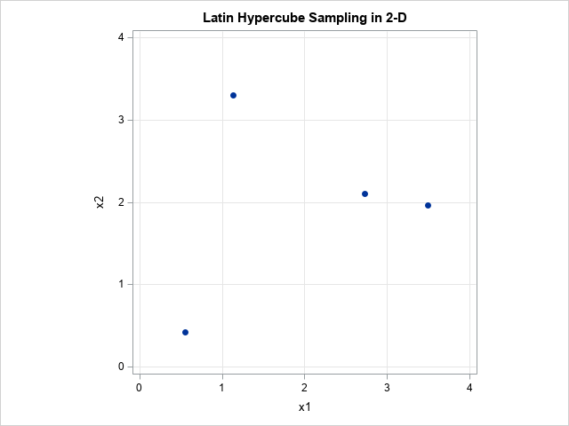
Notice that each variable is divided into four subintervals, so the Cartesian product of the variables is divided into 16 rectangles. Of these, k=4 rectangles contain points. Each row and each column in the grid contains only one point. If you look back at the section about Latin squares, these points are in rectangles that correspond to the positions of the 'A' letters in the 4 x 4 Latin square that PROC PLAN created.

Latin hypercube sampling for five variables

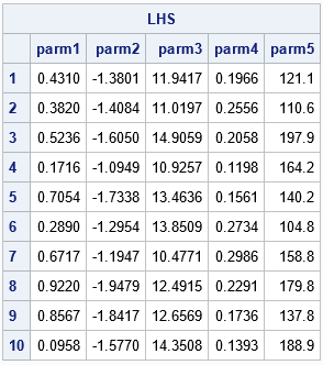
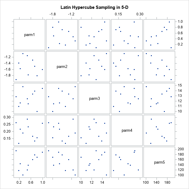
The following call reproduces the second example in Gao (2019), which generates a Latin hypercube sample for five variables that have different ranges. The range of each variable is specified as a row of the 'intervals' matrix. Each range is split into 10 equal-width subintervals. A random point is selected in each subinterval for each variable. Lastly, the Latin sample is returned. The sample contains 10 points in five dimensions. You can use a scatterplot matrix to visualize the sample.

/* 5-D example */
/*           min  max */
intervals = { 0    1,
             -2   -1,
             10   15,
             0.1  0.3,
             100  200};
varNames = 'parm1':'parm5';
LHS = LatinHyperSample(intervals, 10);
print LHS[c=varNames f=BESTD8. r=(1:10)];
 
/* write the sample to a SAS data set */
create lhsEx2 from LHS[c=varNames];
   append from LHS;
close;
QUIT;
 
title "Latin Hypercube Sampling in 5-D";
proc sgscatter data=lhsEx2;
   matrix parm1-parm5 / markerattrs=(symbol=CircleFilled);
run;

Comment on the implementation

The concept of Latin hypercube sampling can be generalized. This implementation splits the range of each variable into k equal-length subintervals. If each variable is distributed uniformly, then the equal-length subintervals are also equi-probable. However, if a variable is distributed non-uniformly, it makes sense to make the subintervals different lengths so that they become equiprobable. You can use quantiles of the underlying distribution to split the range of each variable into equi-probable intervals, then use the inverse CDF method to obtain a random point in each interval.

Summary

This article is inspired by Gao (2019), who showed how to implement Latin hypercube sampling in SAS. This article improves the implementation by making it simpler and more efficient.

Blogs