A colleague asked me an interesting question:

I have a journal article that includes sample quantiles for a variable. Given a new data value, I want to approximate its quantile. I also want to simulate data from the distribution of the published data. Is that possible?

This situation is common. You want to run an algorithm on published data, but you don't have the data. Even if you attempt to contact the original investigators, the data are not always available. The investigators might be dead or retired, or the data are confidential or proprietary. If you cannot obtain the original data, one alternative is to simulate data based on the published descriptive statistics.

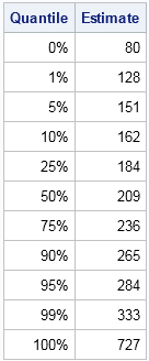
Simulating data based on descriptive statistics often requires making some assumptions about the distribution of the published data. My colleague had access to quantile data, such as might be produced by the UNIVARIATE procedure in SAS. To focus the discussion, let's look at an example. The table to the left shows some sample quantiles of the total cholesterol in 35 million men aged 40-59 in the years 1999–2002. The data were published as part of the NHANES study.

With 35 million observations, the empirical cumulative distribution function (ECDF) is a good approximation to the distribution of cholesterol in the entire male middle-aged population in the US. The published quantiles only give the ECDF at 11 points, but if you graph these quantiles and connect them with straight lines, you obtain an approximation to the empirical cumulative distribution function, as shown below:

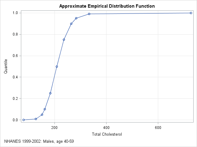
My colleague's first question is answered by looking at the plot. If a man's total cholesterol is 200, you can approximate the quantile by using linear interpolation between the known values. For 200, the quantile is about 0.41. If you want a more exact computation, you can use a linear interpolation program.

The same graph also suggest a way to simulate data based on published quantiles of the data. The graph shows an approximate ECDF by using interpolation to "connect the dots" of the quantiles. You can use the inverse CDF method for simulation to simulate data from this approximate ECDF. Here are the main steps for the simulation:

• Use interpolation (linear, cubic, or spline) to model the ECDF. For a large sample of a continuous variable, the approximate ECDF will be a monotonic increasing function from the possible range of the variable X onto the interval [0,1].
• Generate N random uniform values in [0,1]. Call these values u₁, u₂, ..., u_N.
• Because the approximate ECDF is monotonic, for each value u_i in [0,1] there is a unique value of x (call it x_i) that is mapped onto u_i. For cubic interpolation or spline interpolation, you need to use a root-finding algorithm to obtain each x_i. For linear interpolation, the inverse mapping is also piecewise linear, so you can use a linear interpolation program to solve directly for x_i.
• The N values x₁, x₂, ..., x_N are distributed according to the approximate ECDF.

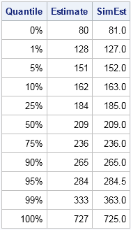
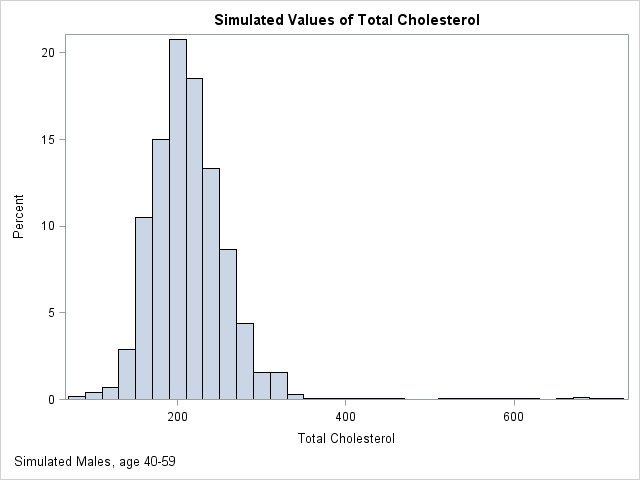
The following graph shows the distribution of 10,000 simulated values from the piecewise linear approximation of the ECDF. The following table compares the quantiles of the simulated data (the SimEst column) to the quantiles of the NHANES data. The quantiles are similar except in the tails. This is typical behavior because the extreme quantiles are more variable than the inner quantiles. You can download the SAS/IML program that simulates the data and that creates all the images in this article.

A few comments on this method:

• The more quantiles there are, the better the ECDF is approximated by the function that interpolate the quantiles.
• Extreme quantiles are important for capturing the tail behavior.
• The simulated data will never exceed the range of the original data. In particular, the minimum and maximum value of the sample determine the range of the simulated data.
• Sometimes the minimum and maximum values of the data are not published. For example, the table might end begin with the 0.05 quantile and end with the 0.95 quantile. In this case, you have three choices:
  • Assign missing values to the 10% of the simulated values that fall outside the published range. They simulated data will be from a truncated distribution of the data. The simulated quantiles will be biased.
  • Use interpolation to estimate the minimum and maximum values of the data. For example, you could use the 0.90 and 0.95 quantiles to extrapolate a value for the maximum data value.
  • Use domain-specific knowledge to supply reasonable values for the minimum and maximum data values. For example, if the data are positive, you could use 0 as a lower bound for the minimum data value.

Have you ever had to simulate data from a published table of summary statistics? What technique did you use? Leave a comment.