A previous article shows how to use PROC FCMP to define the PDF, CDF, and quantile functions for the three-parameter Burr XII distribution. I also defined the log-PDF function, which is used during maximum likelihood estimation (MLE) of parameters. This article shows how to fit the Burr distribution to data in SAS by using MLE. If you have a license for SAS/ETS software, you can use PROC SEVERITY, which has built-in support for the Burr distribution. If you do not have a license, you can use PROC NLMIXED along with the log-PDF function that was defined in the previous article. You could also use the optimization methods in PROC IML.
Define household income data
To demonstrate the fitting process, consider the following sample of 150 observations that represent household income (in thousands of dollars). Household income is a classic application for the Burr XII distribution because it typically exhibits right skewness and a heavy tail.
data HouseholdIncome; input y @@; datalines; 89 142 44 15 65 25 34 29 55 15 95 88 42 49 32 25 53 81 94 51 37 20 54 31 45 25 42 58 50 136 41 25 59 42 32 25 62 55 86 39 56 59 44 54 132 48 37 15 35 64 103 26 59 86 29 59 21 51 35 30 124 148 95 82 52 49 62 23 44 113 54 67 92 67 46 30 33 54 50 99 61 40 99 67 136 56 80 100 15 60 59 102 53 109 55 17 16 75 49 51 15 65 46 94 65 56 52 97 54 44 16 60 147 57 38 52 160 48 104 31 40 43 201 80 51 32 28 64 159 51 14 57 123 8 176 72 26 58 84 17 38 92 51 55 88 10 37 60 71 157 ; proc means data=HouseholdIncome N Min Max Mean Std Skew Kurt ndec=3; var y; run; |
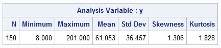
The call to PROC MEANS shows descriptive statistics for the data. The data has positive skewness and heavier-than-normal tails (kurtosis = 1.828). The data shows a wide dispersion (StdDev=36.457) and the range shows that one family earns only $8k whereas another earns more than $200k.
Fit the Burr distribution by using PROC SEVERITY
If you have a license for SAS/ETS software, you can use PROC SEVERITY to estimate the three parameters in the Burr distribution that are most likely, given the data. One of the advantages of PROC SEVERITY is that it automatically provides starting values for the parameter estimates prior to optimizing the loglikelihood function. In the call to PROC SEVERITY, the LOSS statement identifies the response variable, which is Y. The DIST statement specifies one or more distributions to fit.
/* use PROC SEVERITY in SAS/ETS to fit a Burr XII model to data */ proc severity data=HouseholdIncome plots(only histogram)=(pdf); loss y; dist Burr; run; |
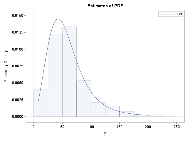
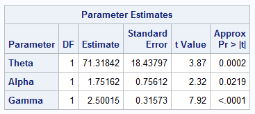
The output provides parameter estimates and standard errors for the Burr parameters. It also provides a graph that overlays a histogram of the data with the density estimate for the fitted Burr distribution.
Fit the Burr distribution by using PROC NLMIXED
If you do not have SAS/ETS software, you can still fit the model by using PROC NLMIXED. This procedure enables you to specify the loglikelihood function. You can specify the function by using programming statements within the body of the procedure, but in this example, I show how to call the logPDF_Burr function that was defined by using PROC FCMP. Before calling PROC NLMIXED, be sure the run the PROC FCMP procedure in the Appendix of the previous article, which defines and stores the logPDF_Burr function.
When using PROC NLMIXED, you must provide two details that PROC SEVERITY handles automatically:
- Initial guesses: The optimization algorithm needs a starting point for the parameters (θ, γ, α). Providing a good guess can be difficult, but fortunately PROC NLMIXED provides a way for you to specify initial guesses on a grid in parameter space. The procedure evaluates the loglikelihood at each point on the grid, then starts the optimization from the parameter values that yields the largest loglikelihood.
- Parameter constraints: Since PROC NLMIXED doesn't know anything about the function it is optimizing, you must use the BOUNDS statement to specify that θ, γ, and α are strictly positive.
/* You can use PROC NLMIXED to fit any distribution, but you need to provide a starting guess and the log-PDF function. The log-PDF function was defined previously in https://blogs.sas.com/content/iml/2026/01/20/burr-sas.html */ options cmplib=work.funcs; /* define location of Burr functions stored by PROC FCMP */ proc nlmixed data=HouseholdIncome; /* specify a grid of values for the initial guesses */ parms theta 36 50 /* sample stddev = 36 */ gamma 1.5 2 2 alpha 2 5 10 / BEST=5; /* display the best 5 values */ bounds theta > 0, gamma > 1, alpha > 1; LL = logPDF_Burr(y, theta, gamma, alpha); model y ~ general(LL); ods exclude IterHistory; run; |
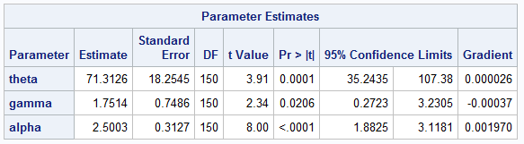
For the scale parameter, θ, I used 36 (close to the sample standard deviation) and 50 for grid values. For the shape parameters, I chose values typical of income distributions. The output shows that PROC NLMIXED found the same local maximum for the loglikelihood as PROC SEVERITY.
Summary
The Burr XII distribution is a model for skewed and heavy-tailed data, especially in economics. PROC SEVERITY in SAS/ETS software includes the Burr distribution as a built-in distribution, which makes it easy to fit the distribution to data. If you do not have a SAS/ETS license, you can use PROC NLMIXED in conjunction with PROC FCMP to obtain parameter estimates by maximizing the loglikelihood function.

1 Comment
Pingback: Implement the Burr distribution in SAS - The DO Loop