A previous article describes the nonnegative matrix factorization (NMF). You can use the NMF to reveal important features in data that can be used to reduce the dimensionality of the problem. NMF is useful when the data are nonnegative, such as counts or pixel values in an image. The goal of NMF is to find a small number of new nonnegative variables that are interpretable and such that each original observation is approximated as a nonnegative linear combination of these new variables. In that sense, NMF shares similarities with principal component analysis (PCA), but the PCA factors and the coefficients contain negative values, which hampers interpretability.

Recently, I read a paper by Patrick Hoyer (2004, "Non-negative matrix factorization with sparseness constraints"), that imposes constraints on the NMF method. The constraints are designed to make the factors more sparse, which is why Hoyer introduced his sparseness measure for vectors. Briefly, Hoyer's algorithm results in nonnegative factors that might be more interpretable.

This article shows an example by revisiting the Scotch whisky data, which I analyzed by using NMF in a previous article. On paper, Hoyer's idea seemed both interesting and powerful. However, after running a sparseness-constrained NMF on an example, I was not impressed. Read on to find out why. To try out the Hoyer algorithm yourself, download the SAS program that implements a sparseness-constrained NMF factorization.

An unconstrained feature set for Scotch whiskies

The previous article used the NMF to extract a four-dimensional basis of vectors for Scotch whisky data. It is known that whiskies often have regional characteristics, such as the "earthy" or "peaty" whiskies from the island of Islay. Ideally, the NMF features would reflect these regional flavor characteristics.

The whisky data can be represented as an 86x12 nonnegative data matrix, X. Each row represents flavor characteristics of a whisky. Each whisky is assigned a flavor profile that consists of the values 0-4 for the 12 flavors. The 12 flavors are Tobacco, Medicinal, Smoky, Body, Spicy, Winey, Nutty, Honey, Malty, Fruity, Sweetness, and Floral.

The NMF creates a rank-k approximation to X. This article uses k=4. Thus, X is approximated as a product W*H, where W is 86x4 and H is 4x12. The rows of H are the "flavor profile" feature vectors. They form a basis for a 4-D linear subspace. They are analogous to the principal components (eigenvectors) in a PCA analysis. Each row of the W matrix is a set of weights (or coefficients) for the 4-factor approximation of the corresponding row of X.

The following image shows the transposed H matrix. The columns in the image visualize a 4-D basis for the unconstrained NMF.

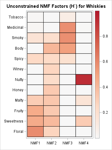
The columns of H` are the features found by the NMF. The NMF method is not unique, but in this image:

1. The first NMF factor is a combination of six flavors: Smoky, Spicy, Malty, Fruity, Sweetness, and Floral variables.
2. The second NMF factor is a combination of 10 flavors.
3. The third factor is primarily composed of the Tobacco, Medicinal, Smoky, and Body flavors.
4. The fourth factor is primarily composed of Nutty flavor, with smaller amounts of Malty and Sweetness.

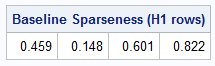
In terms of Hoyer's sparseness measure, the first and second features are not sparse. Hoyer's measure ranges from 0 (not at all sparse) to 1 (very sparse). The following table shows that the first NMF feature has moderate sparseness (0.459). The second feature has very little sparseness (0.148). The third and fourth features are strongly sparse (0.601) and very strongly sparse (0.822), respectively.

Before leaving the visualization of the unconstrained NMF, I want to draw your attention to the first row of H`. The third factor contains a small amount of the Tobacco variable. The cell is light orange. If you print out the H matrix, you can see that the first and second factor also contain a trace amount of the tobacco variable. However, compared to the other variables, this rank-4 NMF approximation does not represent the tobacco variable well. It seems that the tobacco variable probably points in a direction that is primarily orthogonal to the span of these four NMF factors.

A sparseness-constrained NMF algorithm

There are 12 variables and k=4 factors, so it would be nice if features were combinations of no more than four or five variables. If a 12-D vector has 4 nonzero components and 8 zero components, Hoyer's sparseness measure is about 0.6. Let's use that value as a target value. What will the value 0.6 do? The unconstrained factors naturally ranged from 0.15 to 0.82. The sparseness constraint forces the dense factor (0.15) to become much sparser. However, it will actually reduce the sparseness of the fourth factor!

I implemented Hoyer's sparseness-constrained NMF in SAS IML. The following image shows the result of running this constrained NMF algorithm on the Whisky data and constraining the rows of the H matrix to have sparseness equal to 0.6:

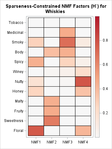
In the new NMF factorization, the sparseness of EVERY feature (rows of the H matrix) is exactly 0.6. In the new factorization, all features depend on 4-5 variables. Notice that the second feature, which used to be a blend of 10 flavors, is very different. Some of the flavors that were previously captured in the second feature are now part of other factors. For example, the Winey contributions have moved to the fourth factor, and the Honey contribution has moved to the first factor.

If you look closely at the first row in the image, you'll see that no factor contains the Tobacco variable! In this rank-4 sparseness-constrained factorization, the sparseness constraint forces the columns of H` to be formed by using only a few variables. The Tobacco variable is not included in any sparse factor. Thus, this model predicts that no Scotch whisky has a Tobacco flavor.

If you want to include the Tobacco variable in the NMF factors, you need to relax the the sparseness constraint (or use a higher-rank approximation). For example, setting the sparseness target to 0.5 will result in factors that include Tobacco, but the resulting factors each contain six or more variables and are not as interpretable.

This is a specific instance of a general truth: The unconstrained NMF factorization will always approximate the data matrix better than a sparseness-constrained factorization. Sometimes, the lack of fit might be qualitatively noticeable, as in this example where the Tobacco variable is not included in any NMF factor.

The tradeoffs between sparseness and goodness of fit

The sparseness-constrained NMF is always a poorer approximation to the data matrix. Thus, you have to decide whether the trade-offs are worth it:

• Is it better to use the unconstrained NMF? The fit is better, but some factors might be formed as a linear combination of many variables, which hampers interpretability.
• Is it better to use the sparseness-constrained NMF? The fit is worse, but you can force the factors to be sparse and therefore highly interpretable. On the other hand, the sparseness constrained NMF is a Procrustean solution to the interpretability of the factors. By forcing every factor to have the same sparseness, it ignores the natural data-induced correlations between variables.

My general preference is to let the data decide how many variables are contained in each NMF factor. The unconstrained NMF approximation seems more faithful to the data. The factors in the unconstrained NMF are mostly interpretable. Their sparseness ranges from 0.148 (not sparse) to 0.822 (strongly sparse). It isn't terrible to have a factor whose interpretation is "an overall blend of flavors." After all, every observation is a Scotch whisky, so it isn't surprising to have a common factor that describes flavors that are common to many whiskies.

In the sparseness-constrained algorithm, every factor has exactly the same sparseness. Every factor depends strongly on four or five flavors. This does not seem realistic. If regional distilleries produce whiskies that have one or two special flavor characteristics, it seems better to have factors that are linear combinations of only one or two flavors. But the sparseness of such a factor would be too high for the specified constraint.

Summary

In multivariate statistics, the best algorithms are often those that let the data decide the features. By adding a sparseness constraint to the NMF algorithm, we let the tail wag the dog. The sparseness essentially dictates how many variables are important in each factor. If the sparseness value is high, then every factor will contain a small number of important variables, which might not be appropriate for the data.

There is also the mathematical fact that a constrained solution will always have a poorer fit than an unconstrained solution. By itself, that doesn't bother me too much, but you should get something valuable for the loss of fit. In a sparseness-constrained NMF, it isn't clear that the benefits offset the poorer approximation to the data.

Appendix: Sparseness and goodness of fit

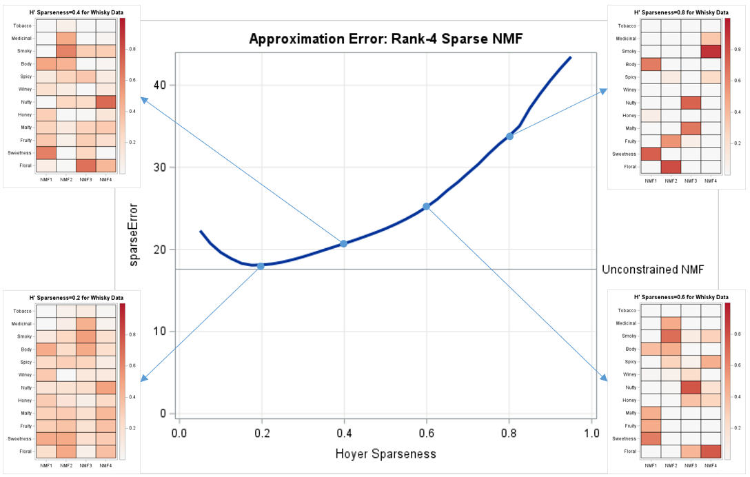
It is an interesting exercise to plot the fit of rank-4 NMF approximation as you let the sparseness constraint vary from small to large values. The following image summarizes that experiment for the Whisky data. I have overlaid a few plots of the H` matrix so that you can see the effect that sparseness has on the NMF factors. The horizontal line is the relative error of the unconstrained NMF. The relative error compares the NMF error E=||X - W*H||_F with the smallest possible error, which is produced by using a rank-k SVD.