This is the last article in a series about computing probabilities for the multivariate normal distribution.
A previous article shows how to compute the probability of a standardized multivariate normal (MVN) distribution in an orthant for dimensions k=1, 2, and 3 by using the Childs-Sun formulas.
The formulas are exact and are expressed in terms of the arcsine of the correlation coefficients of a general correlation matrix.
For example, if X~MVN(0, R) is a standard trivariate normal random variable, the probability that X is in the first orthant
{X | X1 > 0, X2 > 0, X3 > 0}
is given by the formula:
\(P_3 = \frac{1}{8} + \frac{1}{4\pi} \left( \sin^{-1}(R_{12}) + \sin^{-1}(R_{13}) + \sin^{-1}(R_{23}) \right)\)
where R12, R13, and R23 are the off-diagonal elements of a general 3x3 correlation matrix.
You might hope that higher-dimensional Childs-Sun formulas are similarly simple. Alas, they are not! For the higher-dimensional formulas, the probabilities are defined recursively. As the dimension increases, the number of terms explodes combinatorially. This article shows a SAS IML module that implements the Childs-Sun formula for the orthant probability of a 4-D standardized normal distribution. After implementing the 4-D case, I have no desire to attempt higher dimensions!
The Childs-Sun formula for dimension 4
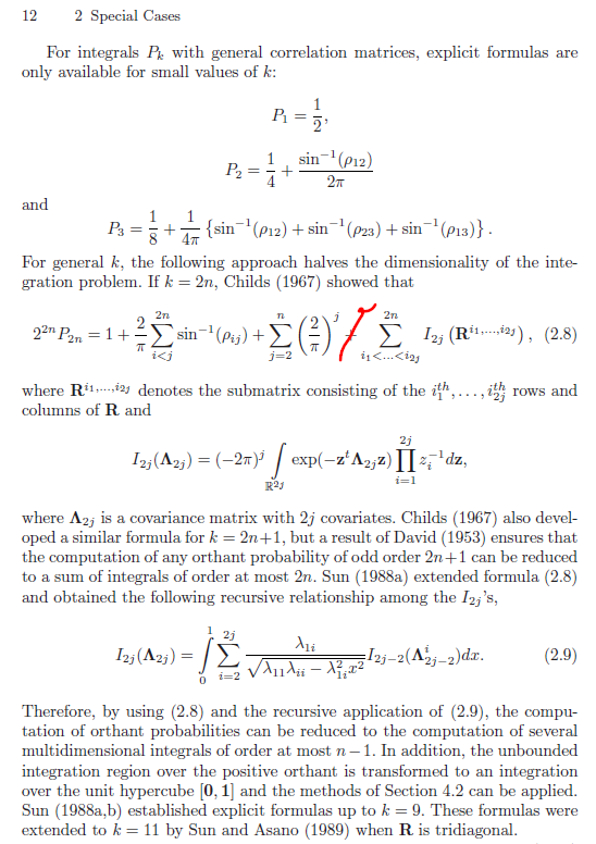
Appendix 1 shows a snippet from p. 12 of Genz and Bretz (2009), which describes the Childs-Sun formula for an MVN orthant probability. The formula relies on the Childs-Sun reduction method (Childs, 1967; Sun, 1988). Similar to the lower-dimensional formulas, the 4-D formula contains a sum of arcsines of the correlation coefficients. However, the formula adds additional terms that involve an integral, I4. The integrands are complicated expressions of the off-diagonal elements of a 4x4 correlation matrix.
In 4-D, there are 16 orthants. As discussed in a previous article, if you can find the probability in the "first orthant" (the one where all components have positive signs), you can use a clever "reflection trick" to find the probability in the other 15 octants.
In Genz and Bretz (2009), the Childs-Sun formula for the orthant probability, which they call P4, has an unfortunate typo. The correct formula is shown in Appendix 1, where the red "delete" symbol removes an erroneous "plus sign." It took me many hours to decipher the notation. By consulting other references (Gehrlein and Saniga (1977); Sun and Asano (1990)), and with some assistance from the Google Gemini AI, I was able to decipher the formulas and create a SAS IML function that evaluates the orthant probability. The IML function is presented in this article.
Conditional probability and the geometry of the formula
I usually explain the mathematical details of my SAS programs, but I'm not going to do that today. The formula is too complicated to describe in a short blog post. Some details are in the original Childs (1967) paper, which is unfortunately behind a paywall.
The general formula (see Appendix 1) is very complicated. But if you restrict to k=4 dimensions (hence, n=2), the formula
looks something like this:
\(P_4 = \frac{1}{16} + \frac{1}{8\pi} \sum_{i < j}^4 \sin^{-1}(R_{ij}) + \frac{1}{4\pi^2} I_4(R)\)
where I4 is a complicated sum of one-variable integrals. Each integral
depends on a lower-dimensional integration, called I2, which is why this is a recursive formula.
The notation is explained further in Appendix 2.
The one-variable integrals are the key. In general, to evaluate the probability of a 4-D distribution, you must solve a 4-D volume integral. The Childs-Sun method uses the geometry of the multivariate normal distribution to reduce this volume to a sum of iterated integrals that accumulate lower-dimensional slices.
This formula is an application of conditional probability. The dummy integration variable, x, is a continuous variable on [0,1]. For a fixed value of x, the term R1i(x) evaluates to a conditional correlation matrix. The variables inside the integrand (e.g., the quadratic denominator w = 1 - R1i2 x2) are conditional variances and partial correlations.
The I2 function evaluates a 2-D orthant probability (which has an exact arcsine solution) for the remaining two variables, given that the other variables are fixed at a slice determined by x. You can use the QUAD subroutine in SAS IML to integrate over x in [0,1], which aggregates these 2-D conditional probabilities to sweep out the exact probability mass of the 4-D volume.
Implementing the P4 formula in SAS IML
The main SAS IML function is called P4_childs, which computes the 4-D orthant probability. It calls the QUAD subroutine to compute I4. The integrand is ProbInt4, which builds terms from the off-diagonal elements of the 4x4 correlation matrix. The DO loop evaluates three different conditional correlation matrices.
proc iml; /* The base case: P2. For a scalar correlation, rho, returning the orthant probability, P2. See https://blogs.sas.com/content/iml/2026/05/11/mvn-orthant-probability.html */ start P2(rho); return( 0.25 + arsin(rho) / (2*constant("pi")) ); finish; /* The sum of the I4 integrands. Instead of evaluating the three integrals separately, evaluate the sum of the integrals and perform one numerical integration. Evaluates the Sun (1988) residual partial correlation matrix. Whereas Genz/Bretz Eqn 2.8-2.9 uses a general covariance matrix, this function assumes R is a correlation matrix, so R[i,i]=1 */ start ProbInt4(x) global(R_global); R = R_global; pi = constant("pi"); x2 = x # x; sum = 0; /* The sum of three terms: i=2, 3, and 4 */ do i = 2 to 4; /* Determine the indices (j, k) of the two remaining variables */ if i=2 then do; j=3; k=4; end; else if i=3 then do; j=2; k=4; end; else do; j=2; k=3; end; /* R_ii term: The quadratic denominator */ w = 1 - R[1,i]##2 * x2; /* R[i,i]=1 for all i */ if w< 1E-12 then w = 1E-12; /* Numerical safeguard */ /* Compute the conditional variances and covariance. These are a_11, a_12, etc, in Sun and Asano */ a_jj = 1 -R[1,j]##2 * x2 -((R[i,j] - R[1,i]*R[1,j]*x2)##2) / w; a_kk = 1 -R[1,k]##2 * x2 -((R[i,k] - R[1,i]*R[1,k]*x2)##2) / w; a_jk = R[j,k] -R[1,j]*R[1,k]*x2 -(R[i,j] - R[1,i]*R[1,j]*x2)*(R[i,k] - R[1,i]*R[1,k]*x2) / w; /* rho is the off-diagonal element of the conditional correlation matrix */ rho = a_jk / sqrt(a_jj * a_kk); /* ensure rho is in [-1,1]. See https://blogs.sas.com/content/iml/2026/02/04/clip-values.html */ rho = ( -1 <> (rho >< 1) ); /* clamp to [-1,1] */ /* Call P2 function to get the I2 term */ I2_val = 2 * pi * ( P2(rho) - 0.25 ); /* this actually simplifies to ARSIN(rho) :-) */ /* Add the i-th term to the sum */ sum = sum + (R[1,i] / sqrt(w)) * I2_val; end; return(sum); finish; /* The main P4 function, which evaluates the Childs-Sun formula for 4 dimensions */ start P4_Childs(R) global(R_global); R_global = R; /* Set the global correlation matrix for QUAD */ /* Integrate ProbInt4 over the interval [0, 1] */ call quad(I4, "ProbInt4", {0 1}); /* Apply the Childs (1967) formula */ pi = constant("pi"); sum_arsin = sum( arsin(R[{2 3 4 7 8 12}]) ); /* sum of arcsine for all 6 off-diagonal elements */ prob = 1/16 + sum_arsin / (8*pi) + I4 / (4 * pi**2); /* fixes the typo in Genz and Bretz, Eqn 2.8 */ return(prob); finish; /* --- Simple Test --- */ R = {1.0 0.5 0.3 0.2, 0.5 1.0 0.4 0.3, 0.3 0.4 1.0 0.5, 0.2 0.3 0.5 1.0}; ans = p4_Childs(R); print ans; |

When you run this code, the exact Childs-Sun formula produces an orthant probability of 0.1611218 for the given matrix.
You can verify that value by using a Monte Carlo simulation. The following Monte Carlo simulation
uses one million random points from the MVN(0, R) distribution. In addition to the
Monte Carlo estimate, I generate a 95% confidence interval for the probability.
/* Use Monte Carlo simulation to estimate the probability that a MVN random variable is less than a specified value in each coordinate. Sigma is a kxk covariance matrix; mu is an option row vector with k elements. The row vector b specifies the upper limits of integration. The function returns an estimate of P(X1<b[1] & X2<b[2] & ... & Xk<b[k] | X~MVN(mu, Sigma)) by simulating N random variates from MVN(mu, Sigma) and returning the proportion that are in the specified region. */ start MC_CDFMVN(N, b, Sigma, mu=j(1,ncol(Sigma),0)); X = randnormal(N, mu, Sigma); inRegion = j(N,1,1); do i = 1 to ncol(b); v = (X[,i] < b[i]); inRegion = inRegion & v; end; return mean(inRegion); finish; N = 1E6; prob_MC = MC_CDFMVN(N, {0 0 0 0}, R); SE_MC = sqrt( prob_MC * (1-prob_MC)/N ); Lower95 = prob_MC - 1.96*SE_MC; Upper95 = prob_MC + 1.96*SE_MC; print prob_MC Lower95 Upper95; |
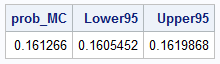
The output from the Monte Carlo simulation shows that the Monte Carlo estimate is close to the value returned by the Childs-Sun formula. In addition, the 95% confidence interval includes the exact value, which gives me "confidence" (pun intended!) that I implemented the Childs-Sun formula correctly. You can repeat the computations for other 4x4 correlation matrices and obtain similar results.
Summary
As my dear mother used to say when faced with a challenging situation, "this is not for the faint of heart." The Childs-Sun formula for the orthant probability of a multivariate normal distribution is a complicated equation. In 2-D and 3-D, it simplifies into a sum of arcsines. In higher dimensions, you must compute conditional correlation matrices and integrate them to evaluate the formula. I have shown a SAS IML function that implements the formula in 4-D.
Despite the complexity, this is an amazing mathematical and computational result! The Childs-Sun formula is an exact analytical solution to a 4-dimensional multivariate normal volume integral over an orthant. And, as shown previously, you can use the P4_Childs function to compute the MVN probability for any 4x4 correlation matrix in any orthant.
Appendix 1: The general Childs-Sun formula for orthant probabilities
The following image is from p. 12 of Genz and Bretz (2009), Computation of Multivariate Normal and t Probabilities. The last term of Eqn 2.8 has a typo in Genz and Bretz. The equation contains a plus sign that should not be there. This typo caused me hours of confusion! I finally cross-referenced the equation with Sun and Asano (1990) and the original article by Childs (1967), which both display the correct equation.
Note the somewhat confusing notation in the Childs-Sun formula. The superscript on the argument to the I2j function describes the submatrix to use in computing the conditional probabilities. This is not explained further in G&B. For the details of the implementation, see the SAS IML function in this article. The superscript on the argument to the I4 function describes the submatrix to use in computing the conditional probabilities. This is not explained further in G&B. For the details of the implementation, see the SAS IML function in this article.
Appendix 2: The sum notation
The Genz and Bretz notation for the sum of integrals is very dense. Here is what it means in the 4-D case. For this case, n=2, which means that the outer sum reduces to j=2. The inner sum looks like
\(\sum_{i_1 < \ldots < i_4}^4 I_4(R^{i_1,\ldots,i_4})\).
The notation is a combination sum. It means, "Sum over all possible combinations of the distinct indices chosen from the set {1, 2, 3, 4} subject to the constraint that the combinations are in increasing order." Well, for four indices, there in only one combination that satisfies this constraint, and it is the tuple (1, 2, 3, 4). So the inner summation also vanishes and becomes I4(R). You can drop the superscript because you are sending in all four columns of the 4x4 matrix, R.
The I4 term is defined recursively in terms of I2. Now the sum matters. When j=1, the summation is
\(\sum_{i_1 < i_2}^4 I_2(R^{i_1,i_2})\).
There are six ways to choose two distinct ordered indices from the set {1,2,3,4}. Since I2(Ri1, i2) = arcsine(R[i1, i2]),
we get the sum-of-arcsine terms
\(\sum_{i < j} \sin^{-1}( R_{ij} )\).
