Stratified bootstrapping and when to use it

When you use the bootstrap method in statistics, the most common resampling method is called case resampling. For data that has N observations, each bootstrap sample is created by sampling with replacement from the N observations (or "cases") in the data. However, if the data set includes categorical variables, it might be necessary to perform stratified resampling instead. This article shows how to perform stratified sampling in SAS and discusses two situations in which stratified sampling is a better way to build bootstrap samples.

When is stratified sampling appropriate?

As stated in the documentation for PROC SURVEYSELECT in SAS, if the population is divided into nonoverlapping subgroups (called strata), you can use stratified sampling to select from each stratum independently. In the bootstrap context, each bootstrap resample will contain subgroups that are the same size as in the original data.

Researchers use stratified sampling to select random samples from the population when they suspect that a variable of interest varies across strata or when there are very small subpopulations that are important to represent in the data. For example, a researcher might suspect that a health outcome depends on race. She knows that about 2.9% of the population identifies as Native American. She is concerned that if she recruits 200 subjects at random, the sample might not haver adequate numbers of Native Americans in the study. By intentionally recruiting Native-Americans for the study, she can ensure that she has data for that subpopulation.

As a rule, if the data are collected by using a stratified sample, then you should use stratified sampling when you bootstrap the data. There are two reasons for this:

The "small subpopulation problem" can affect the statistical estimates in the bootstrap samples. For example, if your data set contain 200 observations and only a few Native Americans, the usual case resampling will result in some bootstrap samples that have ZERO Native Americans in them.
The bootstrap resampling should follow the data-generating process as closely as possible. This applies both to stratified designs and nested designs. For example, if the original data samples students inside classrooms inside schools, the bootstrap samples should be constructed similarly. Using stratified sampling is sometimes called a "design-based sampling" method because each bootstrap sample reflects the design of the study.

A GLM analysis of a small data set in SAS

If you are not familiar with how to bootstrap in SAS, read "The Essential Guide to Bootstrapping." For this article, let's bootstrap a 90% confidence interval for the regression coefficients in a simple linear ANOVA model Y ~ GROUP. We'll first perform a conventional bootstrap analysis, which uses sampling with replacement, then compare that analysis with the results of a stratified bootstrap sampling method.

The example data is small (N=20) and has a response variable (Y) and a categorial variable (Group). The Group variable has three levels: Group='A' (N1=8), Group='B' (N2=4), and Group='C' (N3=8). The following SAS statements create the data and graph the Y variable versus the levels of Group. (The X variable is not used in this article.)

data Sample;
input Group $ x y @@;
datalines;
A 6.2 120.0 A 4.6 108.7 A 3.2 101.4 A 5.0 110.7 
A 6.0 125.3 A 6.9 123.8 A 4.9 126.2 A 5.3 114.7 
B 7.8 149.3 B 6.4 119.5 B 6.1 111.5 B 5.8 111.0 
C 5.9 106.4 C 7.8 96.1  C 6.3 111.1 C 7.4 109.5 
C 6.1 109.5 C 9.2 111.7 C 7.4 114.7 C 6.8 105.5 
;
 
title "Distribution by Group";
proc sgplot data=sample noautolegend;
   vbox y / category=Group nofill;
   scatter x=Group y=y / markerattrs=(symbol=CircleFilled);
run;

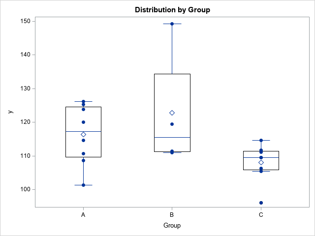
The graph indicates that the mean of the groups differ. The following call to PROC GLM fits coefficients for a simple ANOVA model and uses asymptotic assumptions to estimate a 90% confidence interval for each parameter:

title "ANOVA: Parameter Estimates and CIs";
proc glm data=Sample plots=none alpha=0.1;
   class Group;
   model Y = Group / solution clparm;
quit;

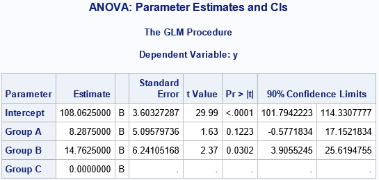
In the GLM analysis, the 'C' group is the reference group. The 90% confidence interval (CI) for the Group='A' coefficient contains 0, but just barely. Because of the small sample size (especially in Group 'B'), you might decide that asymptotic confidence intervals are not suitable. An alternative is to use a bootstrap analysis to estimate the confidence intervals as the percentiles of the parameter estimates from a large number of ANOVA models run on bootstrap resamples.

A review of conventional bootstrap sampling in SAS

I have previously discussed how to perform case resampling to bootstrap a regression model in SAS. You can use the METHOD=URS option on the PROC SURVEYSELECT statement to generate 1,000 bootstrap samples from the data:

%let NumSamples = 1000;       /* number of bootstrap resamples */
 
/* Conventional case resampling for generating bootstrap samples.
   If you do not use the STRATA statement, the number of observations
   for each level of the categorical variables will vary in the bootstrap samples */
proc surveyselect data=Sample NOPRINT seed=123
     method=urs              /* resample with replacement */
     samprate=1              /* each bootstrap sample has N observations */
     OUTHITS                 /* use OUTHITS option to suppress the frequency var */
     reps=&NumSamples        /* generate NumSamples bootstrap resamples */
     out=BootCases(rename=(Replicate=SampleID));
run;
 
/* perform the conventional bootstrap analysis where the num obs for each level varies */
title "Bootstrap Distribution of Regression Estimates: Case Resampling";
ods select none;
proc glm data=BootCases plots=none;
   by SampleID;
   class Group;
   model Y = Group / solution;
   ods output ParameterEstimates = PECases_long;
quit;
ods select all;
 
proc means data=PECases_long mean stddev P5 P95;
   class Parameter;
   var Estimate;
   ods output Summary=Case_summary;
run;

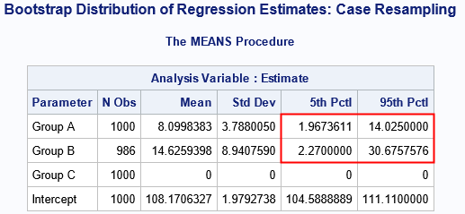
In the bootstrap estimates of the CIs, the CI for the Group='A' coefficient does not contain 0. In addition, the CI for the Group='B' coefficient is considerably wider than the interval CI estimate from PROC GLM.

Notice that the output from PROC MEANS reports that the Group='B' statistics are computed by using 986 observations, not 1,000! That is because 14 samples do not contain any observations from Group 'B'. This is explained further in the next section.

Bootstrap estimates on small subgroups

The output from PROC MEANS indicates that 14 bootstrap samples do not contain any observations from Group 'B'. Let's look more closely at the size of the 'B' subgroup in the bootstrap samples.

The original data has four observations in the 'B' subgroup. In the output data set (BootCase), there are 1,000 samples of size 20. Among the bootstrap samples, the number of observations in the 'B' subgroup will vary. In some samples, the 'B' subgroup will contain 4 observations, whereas other samples might have subgroups of size 3 or 5. The following graph shows the proportion of samples for which the 'B' subgroup contains 0, 1, 2, ..., 11 observations.

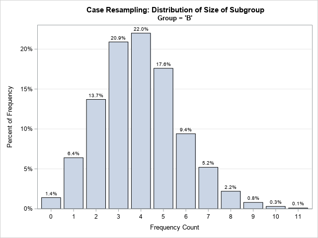
A few bootstrap samples (14 out of 1,000, or 1.4%) do not contain any observations from group 'B'. The Appendix shows how to use elementary probability theory to prove that, in general, you should expect about 1.15% of the bootstrap samples to contain zero observations from group 'B'. So, this example is in agreement with theory.

Stratified bootstrap sampling in SAS

If you used stratified sampling, every sample contains eight observations from the 'A' and 'C' groups and four observations from the 'B' group. Let's see how to implement stratified sampling in SAS.

The first step is to sort the original data by the stratification variables. The STRATA statement is like the BY statement: it causes the SURVEYSELECT procedure to do the same thing (resample) for every level of the categorical variable(s) that you list on the STRATA statement. Let's demonstrate this fact by generating 1,000 bootstrap samples by using case resampling:

/* to use the STRATA statement in PROC SURVEYSELECT, sort the data by the categorical variables */
proc sort data=Sample;
   by Group;  /* put other categorical variables here, if necessary */
run;
 
/* If you want to preserve the number of obs in each level of one or more categorical
   variables, list the variables on the STRATA statement */
proc surveyselect data=Sample NOPRINT seed=123
     method=urs              /* resample with replacement */
     samprate=1              /* each bootstrap sample has N observations */
     OUTHITS                 /* use OUTHITS option to suppress the frequency var */
     reps=&NumSamples        /* generate NumSamples bootstrap resamples */
     out=BootDesign(rename=(Replicate=SampleID));
strata Group; /* put other categorical variables here, if necessary */
run;
 
/* to perform BY-group processing, sort the data by the SampleID variable */
proc sort data=BootDesign;
   by SampleID Group; /* put other categorical variables here, if necessary */
run;
 
/* perform the bootstrap analysis where the num obs for each level is always the same */
title "Bootstrap Distribution of Regression Estimates: Stratified Resampling";
ods select none;
proc glm data=BootDesign plots=none;
   by SampleID;
   class Group;
   model Y = Group / solution;
   ods output ParameterEstimates = PEDesign_long;
quit;
ods select all;
 
proc means data=PEDesign_long mean stddev P5 P95;
   class Parameter;
   var Estimate;
   ods output Summary=Design_summary;
run;

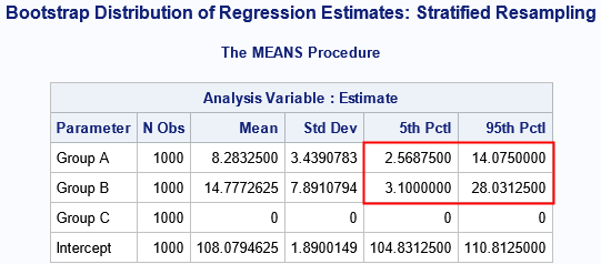
In this analysis, every bootstrap sample contains exactly four observations from Group 'B'. You can see that the bootstrap estimate of the 90% CI is based on 1,000 samples, not 986 as in the previous analysis. In addition, the stratified estimates result in smaller CIs because there is less variation in the size of the subsets.

Summary

This article discusses bootstrap sampling when the data contains categorical variables that represent subpopulations. If you think that the characteristics of the data vary in the subpopulations, you might want to use stratified sampling within the subgroups instead of a sampling method that allows the size of the subgroups to vary among the bootstrap samples. If the data has one or more small subgroups, stratified sampling eliminates the situation where some bootstrap samples contain ZERO observations from the small subgroup.

Appendix: The proportion of bootstrap samples that will contain no observations for a subset

Recall that Group='B' has four observations and the entire data is size N=20. Thus, Group 'B' accounts for 4/20 = 1/5 of the observations. Question: If you select 20 observations from the data at random with replacement, what is the probability that the data does not contain ANY of the observations from Group='B'?

Let's compute the answer. The probability is 1/5 that the first observation is chosen from GROUP='B', so the probability is 4/5 that the first observation is NOT from 'B'. Because we sample with replacement, the probability is the same for every other observation that you select. By independence of the process, the probability is (4/5)²⁰ ≈ 0.0115 that the sample does NOT contain an observation from the 'B' group.

That is a small probability. However, in a bootstrap analysis, we don't generate only one bootstrap sample, we generate a large number such as 1,000 or even 10,000. If you generate a large number of bootstrap samples by using sampling with replacement, you should expect 1.15% of them to not contain any observations from group 'B'.

Blogs