Many people have an intuitive feel for residuals in least square models and know that the sum of squared residuals is a goodness-of-fit measure. Generalized linear regression models use a different but related idea, called deviance residuals. What are deviance residuals, and how can you compute them?

Deviance residuals (and other deviance-based statistics) are produced automatically by SAS regression procedures such as PROC GENMOD. The deviance (defined later) is based on the loglikelihood function for the regression model, so writing down a formula for the deviance can be nontrivial. Fortunately, the SAS DATA step supports the DEVIANCE function, which is a convenient way to compute deviance statistics? The documentation lists several probability distributions (such as normal, gamma, and binomial) for which you can compute the deviance. This article discusses deviance-based statistics in generalized linear models. It also show how to use the DEVIANCE function to reproduce those statistics.

Residuals and least-square models

Most data analysts are familiar with ordinary residuals for linear least-squares regression models. The model is fit to data of the form (y_i, x_i), where x_i represents a row vector of explanatory variables. The model produces a predicted mean μ_i at each value x_i. The residuals are defined as r_i = y_i - μ_i. The residual sum of squares (also called the sum of squared errors (SSE)) is the sum Σ (y_i - μ_i)².

You can use a regression procedure such as PROC GLM to obtain residuals and the residual sum of squares for a regression model. The following DATA step simulates 20 observations from a normal N(10,3) distribution. The call to PROC GLM fits an intercept-only model to the data. The output includes the error sum-of-squares statistic in the OverallANOVA table. To verify that these are the sum of the squared residuals, you can write the residuals to a SAS data set and use PROC MEANS and the USS option to compute the sum of squares for the residuals, as follows:

/* simulate data from a univariate normal distribution */
data SimNormal;
call streaminit(12345);
mu = 10;
do i = 1 to 20;
   y = rand("Normal", mu, 3);
   output;
end;
keep y;
run;
 
proc glm data=SimNormal plots=none;
   model y = ;
   output out=GLMOut residual=resid;
   ods select OverallANOVA ParameterEstimates;
quit;
 
proc means data=GLMOut USS;   /* confirm the sum of squared residuals */
   var resid;
run;

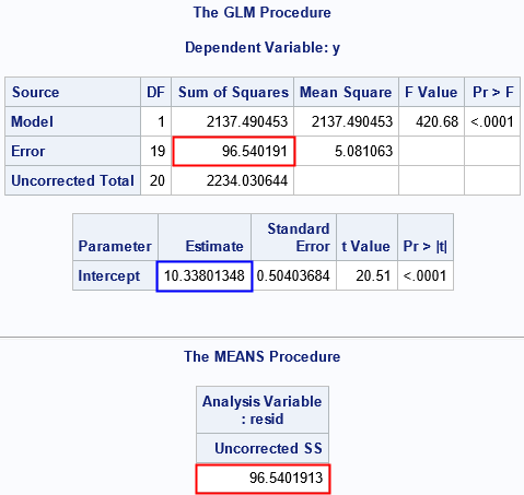
I have highlighted certain statistics in the output. The red box in the GLM output is the sum-of-squared errors (SSE) statistic. The blue box is the estimate of the sample mean (intercept), which is close to the mean of the parent population. The other red box is the manual computation of the sum of the squared residuals. This computation agrees with the output of PROC GLM. The sum of squared residuals (divided by the degrees of freedom) estimates the variance of the residuals. In that sense, the SSE statistic tells us about the variance or dispersion of the residuals.

Deviance residuals

To generalize the concept of a residual, define the deviance in a least-squares model to be the observation-wise statistic d_i = (y_i - μ_i)². With this definition, you can define the deviance residual to be r_i = sqrt(d_i)*sign(y_i - μ_i), which matches the traditional definition. The quantity sqrt(d_i) is the magnitude of the residual.

Why would you want to do this? Because this definition of a (deviance) residual is valid for generalized linear models such as logistic regression, Poisson regression, gamma regression, and more. The formula used for the deviance itself varies according to the type of regression, but the formula r_i = sqrt(d_i)*sign(y_i - μ_i) can now be used for many kinds of regression models. You can use DEVIANCE function in the DATA step to compute the deviance statistic for six different common regression models. As shown in the documentation, each model has a different formula that is used to compute the deviance.

Let's try using the DEVIANCE function for a least squares model. The least squares model assumes normally distributed errors, so you can specify "NORMAL" as the first parameter to the DEVIANCE function to obtain the squared residual value (y_i - μ_i)². For the intercept-only model, all predicted values are the same and equal the mean of the response variable. The following DATA step computes the deviance residuals for the intercept-only model that was analyzed by using PROC GLM:

proc sql noprint; 
   select mean(y) into :mean from SimNormal; /* put the sample mean into a macro variable */
quit;
%put &=mean;
 
data Deviance;
set SimNormal;
d = deviance("Normal", y, &mean);  /* d = (y_i -  mean)**2 */
run;
 
proc means data=Deviance sum;  /* sum of the deviance */
   var d;
run;

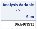
The output from PROC MEANS is the sum of the deviances. Notice that this equals the SSE statistic produced by PROC GLM.

Deviance for other regression models

You can use the GENDOM procedure to fit generalized linear models by using maximum likelihood estimation. For example, the following call to PROC GENMOD fits the same regression model as in the previous section. However, the goodness-of-fit statistic are now given in terms of the sum of the deviance statistics.

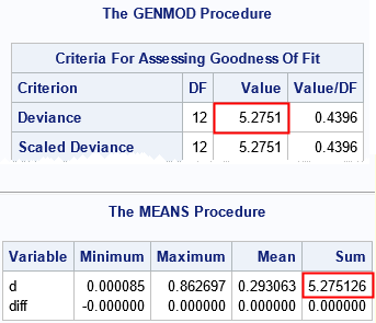
proc genmod data=SimNormal;
   model y =  / dist=Normal;
   output out=GMNorm resdev=resdev pred=pred;
   ods select ModelFit;
run;
 
/* use the DEVIANCE function in the DATA step to reproduce the 
   deviance residuals: resdev_i = sqrt(d)*sign(y_i - mean)
*/
data Check;
set GMNorm;
d = deviance("Normal", y, pred);
resdev2 = sqrt(d)*sign(y - pred); /* manually reproduce the deviance residual */
diff = resdev - resdev2;          /* difference should be 0 for all obs */
run;
 
proc means data=Check ndec=6 min max mean sum nolabels;
   var d resdev resdev2 diff;
run;

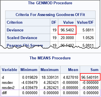
The output from PROC GENMOD includes a table of goodness-of-fit statistics. The first row contains the sum of the deviance statistics (outlined in red). This is the same number as the SSE statistic in PROC GLM. You can confirm that the statistic is correct by using the DATA step and the DEVIANCE function, as shown. The call to PROC MEANS shows that the sum of the deviance statistics is the same as output by PROC GENMOD. Furthermore, the DATA step also manually creates the deviance residual by applying the definition. The DIFF variable is the difference between the manual computation and the deviance residuals from PROC GENMOD. The difference is identically 0.

Deviance residuals for life data

The PROC GENMOD documentation includes an example that models life data by using a gamma distribution. The documentation defines the LIFDATA data and uses the following call to PROC GENMOD to fit a gamma regression model:

proc genmod data = lifdat;
   class mfg;
   model lifetime = mfg / dist=gamma link=log;
   output out=GMGam resdev=resdev pred=pred;
   ods select ModelFit;
run;
 
/* use the DEVIANCE function in the DATA step to reproduce the deviance residuals */
data Check;
set GMGam;
y = lifetime;                     /* the response variable */
d = deviance("Gamma", y, pred);   /* the deviance for a gamma distribution */
resdev2 = sqrt(d)*sign(y - pred); /* manually reproduce the deviance residual */
diff = resdev - resdev2;          /* difference should be 0 for all obs */
run;
 
proc means data=Check ndec=6 min max mean sum nolabels;
   var d diff;
run;

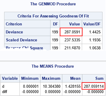
This model includes a classification variable. Nevertheless, the computation of the deviance residuals for the gamma model is similar to the computation in the previous section. The only difference is that "GAMMA" is used as the first argument to the DEVIANCE function. The formula for the deviance for a gamma-distributed errors is more complex than for normally distributed errors, but the DEVIANCE function hides that complexity.

Deviance residuals for binomial regression

The PROC GENMOD documentation includes an example that models binomial data by using a logistic regression model for the proportion of successes among each group in a clinical trial. The following DATA step and call to PROC GENMOD are explained in the documentation:

/* First example in PROC GENMOD doc: Logistic Regression */
data drug;
   input drug$ x r n @@;
   datalines;
A  .1   1  10   A  .23  2  12   A  .67  1   9
B  .2   3  13   B  .3   4  15   B  .45  5  16   B  .78  5  13
C  .04  0  10   C  .15  0  11   C  .56  1  12   C  .7   2  12
D  .34  5  10   D  .6   5   9   D  .7   8  10
E  .2  12  20   E  .34 15  20   E  .56 13  15   E  .8  17  20
;
 
proc genmod data=drug;
   class drug;
   model r/n = x drug / dist=binomial link=logit;
   output out=GMBinom resdev=resdev pred=pred;
   ods select ModelFit;
run;
 
/* use the DEVIANCE function in the DATA step to reproduce the deviance residuals */
data Check;
set GMBinom;
/* pred is the predicted  probability. Convert to expected count */
d = deviance("Binom", r, n*pred, n); /* the deviance for a binomial distribution */
y = r / n;                           /* proportion of successes */
resdev2 = sqrt(d)*sign(y - pred);    /* manually reproduce the deviance residual */
diff = resdev - resdev2;             /* difference should be 0 for all obs */
run;
 
proc means data=Check ndec=6 min max mean sum nolabels;
   var d diff;
run;

The DEVIANCE function for a binomial distribution requires more parameters than for other distributions. Use the second and fourth parameters to specify the number of observed successes and the number of trials, respectively, The third parameter is the expected number of success, which is n*p, where p is the probability of success. The deviance residual is computed by using the difference between the observed and predicted probability of success. Again, the manual computation of the sum of the deviance matches the PROC GENMOD output.

Summary

The parameters for generalized linear models are fit by using maximum likelihood estimation. The deviance is based on the loglikelihood function for the model. The deviance statistic is a goodness of fit statistic, and the deviance residuals are a generalization of the familiar least squares residuals. You can use the DEVIANCE function in the DATA step to compute the deviance statistic and the deviance residuals. The DEVIANCE function is much easier and clearer to use than the explicit formulas for the deviance.