In SAS, the easiest way to draw random sampling from data is to use PROC SURVEYSELECT or the SAMPLE function in SAS IML software. I have previously written about how to implement four common sampling schemes by using PROC SURVEYSELECT and the SAMPLE function.

The DATA step in SAS is also a powerful tool for creating a random sample from data. On discussion forums, when SAS programmers ask about how to generate a random sample, the answers often suggest using the DATA step. For certain sampling methods, the DATA step can be an efficient choice for creating a random sample from existing data. In addition, these sampling methods provide an opportunity to learn some cool features of the SAS DATA step!

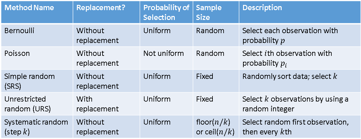
However, sometimes people propose DATA steps programs that are incorrect, inefficient, or confusing. This article clarifies some of the issues and describes how to use the DATA step to implement five sampling methods:

• Bernoulli sample: a random sample without replacement where each observation has an equal probability of being selected. The size of the sample is random.
• Poisson sample: a random sample without replacement where each observation has a specified probability of being selected. The size of the sample is random.
• Simple random sample (SRS): a random sample without replacement where each observation has an equal probability of being selected. The size of the sample is fixed.
• Unrestricted random sample (URS): a random sample with replacement that uses an equal probability at each selection step. The size of the sample is fixed.
• Systematic random sample: Specify an integer k that is much smaller than the sample size, n. Choose a random observation from among the first k, then sequentially choose every k_th observation. The size of the sample is either floor(n/k) or ceil(n/k).

A tabular depiction of these methods is shown in the following table:

Specify uniform probability in the DATA step

Before introducing the sampling methods, it is helpful to review several equivalent ways to specify random selection in the SAS DATA step by using the RAND function.

To select an observation with probability p, you can use either the uniform distribution or the Bernoulli distribution.

• To use the uniform distribution, generate a random uniform variate, u, and compare it to p. Select the observation if u < p.
• To use the Bernoulli distribution, generate a random binary variate from the Bernoulli distribution with probability p. Select the observation if the variate is 1.

Thus, the following two statements are equivalent. To select an observation with probability p, you should select observations for which b equals 1.

   b = ( rand("Uniform") < p );        /* u ~ U(0,1) and u < p */
   b = rand("Bernoulli", p);           /* b ~ Bern(p)  */

Another common expression is generating a random integer in the range 1–N. The modern method is to use the "Integer" distribution. However, you will often see an equivalent formula that uses the uniform distribution in conjunction with the CEIL function. The following SAS statements are equivalent. Each generates a random integer in the range 1–N:

   x = rand("Integer", 1, 20);         /* x ~ UniformInteger(1,20) */
   x = ceil(rand("uniform", 0, 20));   /* u ~ Unif(0,20) */
   x = ceil(20*rand("uniform"));       /* u ~ U(0,1) */

Lastly, I like to remind SAS programmers that they should always use the RAND function for generating random numbers. The older random number functions (RANUNI, RANNOR, UNIFORM, NORMAL, ....) have inferior statistical properties and are deprecated as of SAS 9.4M5.

Example data

The Sashelp.cars data has 428 observations and 15 variables. To make the random samples easier to understand, the following DATA step copies three of the variables from the Sashelp.cars data and creates a new variable that identifies the row of each observation in the data. The new data set is called 'Have':

data Have;
keep OrigObs Make Model Type;
OrigObs = _N_;
set sashelp.cars;
run;

Select a Bernoulli sample

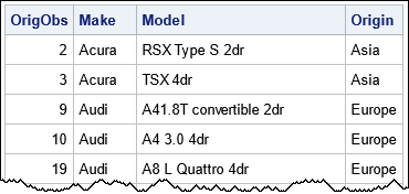
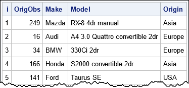
A Bernoulli sample is a random sample without replacement where each observation has an equal probability of being selected. The size of the sample is random. The following example uses the DATA step to create a Bernoulli random sample without replacement from the 'Have' data, where each observation is selected with probability p=0.1.

/* Bernoulli sample : Each obs selected with probability p */
data BernoulliSample;
p = 0.1;               /* choose 0 < p < 1 */
call streaminit(123);
set Have;
if rand("Bernoulli", p);
run;

The following table shows a few rows of the resulting random sample:

Equivalently, you can generate random variates from the uniform distribution, as follows:

data BernoulliSample;
p = 0.1;               /* choose 0 < p < 1 */
call streaminit(123);
set Have;
if rand("Uniform") < p;
run;

Both samples contain the same 48 observations, but if you change the random number seed (in the STREAMINIT call), the size of the sample might be different. If the data set has n observations, the expected size of the sample is p*n. Because the Have data contains 428 observations, this sample has more observations than expected. Notice that the observations in the sample have the same relative order as in the original data.

Select a Poisson sample

A Poisson sample is a random sample without replacement where each observation has a specified probability of being selected. The size of the sample is random.

Sometimes the data set contains a variable that specifies the probability of being selected. Another common situation is that the data contains several groups, and you specify the the probability of selecting an observation from each group. For example, the following DATA step creates a random sample from the 'Have' data where the probability of selecting each observation depends on the value of the 'Origin' variable. The probability of selecting an observation for Origin='Asia' is 0.4, the probability of selecting an observation for Origin='Europe' is 0.2, and the probability of selecting Origin='USA' is 0.3.

/* Poisson sample : Each obs selected with specified probability */
data PoissonSample;
call streaminit(123);
set Have;
 
/* select based on group membership */
if Origin = 'Asia' then prob = 0.4;
else if Origin = 'Europe' then prob = 0.2;
else if Origin = 'USA' then prob = 0.3;
else prob = 0; 
 
u = rand("Uniform");
if u < prob;         /* or,  if rand("Bernoulli", prob); */
run;

The following table shows a few rows of the resulting random sample:

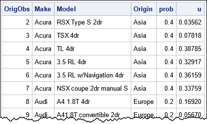
Notice that the observations in the sample have the same relative order as in the original data. The sample has 129 observations. In many situations, you can compute the expected size of the sample. For example, the three levels of the Origin variable have cardinality 158, 123, and 147, so the expect sample size is 0.4*158 + 0.2*123 + 0.3*147 = 131.9.

Select a simple random sample

A simple random sample (SRS) is a random sample without replacement where each observation has an equal probability of being selected. The size of the sample is fixed. If someone tells you they want to "select k observations at random," they often mean that they want a simple random sample from the data.

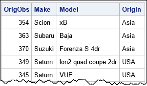
One way to obtain an SRS is to use the DATA step in conjunction with PROC SORT. You use the RAND function to add a uniform random variate to the data, then sort by that variate. You can then select the first k observation in the sorted data. (You might choose to DROP the uniform random variate after sorting.) For example, the following example selects 10 observations at random from the 'Have' data.

/* SRS : Select k=10 obs with equal probability */
data AddUniform;
call streaminit(123);
set Have;
_u = rand("Uniform");
run;
 
proc sort data=AddUniform; by _u; run;
 
data SimpleRandomSample;
set AddUniform(obs=10);    /* select k=10 */
drop _u;
run;

The following table shows a few rows of the resulting random sample. Notice that the observations in the sample do not have the same relative order as in the original data.

Select an unrestricted random sample

An unrestricted random sample (URS) is a random sample with replacement that uses an equal probability at each selection step. The size of the sample is fixed. The following DATA step randomly samples 10 observations with replacement from the 'Have' data:

/* URS */
data SampleWithReplacement;
    retain i k;
    call streaminit(123);
    do i = 1 to 10;
        k = rand("Integer", 1, N);
        set Have point=k nobs=N;
        output;
    end;
    stop;
run;

This program needs an explanation. When the DATA step compiles, it sees a SET statement. It does some preliminary steps to set up running the program. Part of the set-up is to process the two options, POINT= and NOBS=. The POINT= option creates a temporary variable, k. The NOBS= option creates a temporary variable, N, and fills that variable with the number of observations in the 'Have' data set. As temporary variables, neither of these variables will be written to the output data set.

Inside the DO loop, the RAND function generates a random integer in the range 1–N, where N is the size of the data. The program then uses the POINT= option on the SET statement to obtain the k_th observation, which is written to the output data set by the OUTPUT statement.

Recall that when you use the SET statement and sequential access of the data, the DATA step executes an implicit loop over the observations in the input data set. The implicit loop terminates when the DATA step encounters an end-of-file token, which happens after reading the last observation. However, when you use the POINT= option, you are not using sequential access, you are using random access. When you use random access, the DATA step never encounters an end-of-file token, so the implicit loop never exits. This can lead to an infinite loop (and filling up all the disk space!), which is why you should use a STOP statement after using random access. In this case, the STOP statement forces the DATA step to exit after reading 10 observations.

For this example, the sample does not contain any repeated observations. However, for a larger URS, you can select the same observation multiple times.

Select a systematic random sample

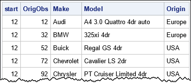
To obtain a systematic random sample, first specify an integer k that is much smaller than the sample size, n. Choose a random observation from among the first k, then sequentially choose every k_th observation. The size of the sample is either floor(n/k) or ceil(n/k). The following DATA step generates a systematic random sample from the 'Have' data for k=20. If selects a random initial observation, then selects every 20th observation after it.

data SystematicSample;
   call streaminit(123); /* Set the random number seed */
   retain first;
   set Have;
   if _N_ = 1 then
      first = rand("Integer", 1, 20);  /* select a starting position */
   if mod(_N_ - first, 20) = 0;        /* select 'first' and every 20th obs after */
run;

You can also generate a systematic sample by using the POINT= option on the SET statement and looping from FIRST to the end of the data set. But the previous program is simpler.

Summary

This article shows five ways to generate random samples from data by using the DATA step in SAS. The examples cover the following methods:

• Bernoulli sample: a random sample without replacement that uses equal probability. The size of the sample is random.
• Poisson sample: a random sample without replacement that uses unequal probability. The size of the sample is random.
• Simple random sample (SRS): a random sample without replacement where the size of the sample is fixed.
• Unrestricted random sample (URS): a random sample with replacement where the size of the sample is fixed.
• Systematic random sample: Select a random observation and every k_th observation after.