A previous article shows that you can run a simple (one-variable) isotonic regression by using a quadratic programming (QP) formulation. While I was reading a book about computational geometry, I learned that there is a connection between isotonic regression and the convex hull of a certain set of points. Whaaaaat? That statement is so unexpected that I felt compelled to verify the result in SAS! This article discusses the connection between the quadratic optimization problem and a convex hull.

The computation uses the cumulative sum of the response values (after sorting by the X values), so the next section discusses a cumulative sum (CUSUM) and the cumulative sum diagram (CSD).

Cumulative sums in statistics

Cumulative sums occur frequently in statistics. For example, in quality control, the CUSUM chart is a graphical technique that enables you to monitor the deviation in a manufacturing process. Various areas of statistics also use CUSUM tests. For example, there is a CUSUM test for testing whether a binary sequence (like a coin toss) is random and there is a CUSUM test in time series analysis that can help to identify a misspecified model.

It is easy to compute cumulative sums in the SAS DATA set or by using the CUSUM function in SAS IML. For example, a previous article used the following data for explaining isotonic regression. In the context of isotonic regression, the data must be sorted by the X variable. You can then use the SAS data step to form the cumulative sum of the response variable. For simplicity, I'll assume no missing values in the data.

/* example data has 19 observations */
data Have;
set sashelp.class;
x = Height;
y = Weight;
keep x y;
run;
 
proc sort data=Have;
   by x;
run;
 
data CSD;      /* CSD = cumulative sum diagram */
retain i s 0;
output;        /* add (i,s) = (0,0) as the initial point */
set Have;
i + 1;         /* enumerate the sequence */
s + y;         /* s is the cumulative sum */
run;

You can graph the cumulative sum of the response variable against the order of the X variable. This is called the cumulative sum diagram (CSD):

title "Cumulative Sum Diagram";
proc sgplot data=CSD;
   series x=i y=s / markers;
   xaxis grid;
   yaxis grid;
run;

On p. 175 of Prepararata and Shamos (Computational Geometry: An Introduction, 1985), they quote a result in Barlow, Bartholomew, Bremner, and Brunk (Statistical Inference Under Order Restrictions, 1972) that states a relationship between the lower convex hull of the cumulative sum diagram and the parameter estimates in isotonic regression. They state that the slopes of the lower convex hull of the CSD are exactly the optimal parameter estimates for the isotonic regression!

Although surprising, this actually has a intuitive statistical interpretation when you think about it. The slope of the i_th line segment in the CSD is exactly y_i because the horizontal distance between each segment is 1. So, the slopes of the lower convex hull will be an average of multiple line segments: $\frac{1}{k} \sum_{j=i}^{i+k} y_j$. This is a running mean. So, intuitively, the convex hull is going to divide the data into blocks of observations. For each block, the best estimate for the piecewise constant isotonic regression line is a running mean of the responses in the block. The surprising fact is that the convex hull of the CSD gives the optimal solution.

Slopes of the lower convex hull

There are two ways to get a convex hull in SAS. In two-dimensions, you can use the CVEXHULL function in SAS IML software. This function is available in SAS 9 and in SAS Viya. For higher dimensions, you can use the CONVEXHULL subroutine, which was released in SAS IML as part of SAS Viya 2023.04. I will use the older CVEXHULL function.

The previous section created the 'i' and 's' variables for the CSD. You can read those variables into SAS IML and compute the convex hull. You can use the DIF function to compute the slopes of the line segments. The following SAS IML program computes the slopes and merges that information with the original data for plotting:

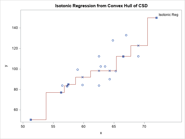
proc iml;
use CSD;
   read all var {'i' 's'} into sites;  /* pts on cumulative sum diagram */
   read all var 'x';                   /* original X coordinates */
close;
 
indices = cvexhull(sites);
k = indices[loc(indices>0)];        /* get vertices on the convex hull */
xCH = sites[k, 1];                  /* get (x,y) coordinates of CH for CSD */
yCH = sites[k, 2];
pred = dif(yCH) / dif(xCH);         /* slopes of the lower convex hull of the CSD */
x = x[k];
*print x pred;                      /* (x,pred) for isotonic regression */
 
create IsotonicReg from x pred [c={'x' 'pred'}];
   append from x pred;
close;
QUIT;
 
data Want;
set Have IsotonicReg;    /* merge with original data */
run;
 
title "Isotonic Regression from Convex Hull of CSD";
proc sgplot data=Want noautolegend;
   scatter x=x y=y;
   step x=x y=pred / markers markerattrs=(symbol=x) JUSTIFY=center lineattrs=GraphData2 curvelabel="Isotonic Reg";
   yaxis label="y";
run;

To me, the most impressive part of this result is how easy it is to implement. I previously solved this problem by using quadratic optimization. Setting up the QP optimization problem involves a dozen lines of code to define the linear and quadratic coefficients and the system of constraints to enforce an isotonic solution. It requires formulating the QP problem in terms of matrices and vectors. In contrast, the convex hull method requires relatively little programming effort to obtain the same solution.

Summary

There are many ways to fit a one-dimensional isotonic regression model to data. Previous articles showed that you can formulate the regression problem as a solution to a quadratic programming (optimization) problem. But a remarkable relationship exists between the isotonic estimates and the slopes of the (lower) convex hull of the cumulative sum diagram of the data. This article uses SAS to compute the convex hull for an example and overlay the isotonic regression curve on the data.