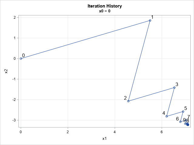
A colleague remarked that my recent article about using Jacobi's iterative method for solving a linear system of equations "seems like magic." Specifically, it seems like magic that you can solve a certain class of linear systems by using only matrix multiplication. For any initial guess, the iteration converges to the solution of the system, as shown in the figure to the right for a two-variable example.
The method is not magical, it is "mathe-magical"! In hopes of finding a simple description of Jacobi's method, I searched the internet for queries such as "Why does Jacobi's method work?", "What is the intuition behind Jacobi's method?", and "What is the geometry of Jacobi's method?" The online web sites that I found were heavy on math, so this article attempts answers those questions in simple prose. I also illustrate the geometry of Jacobi's method for a 2 x 2 example as a way of explaining the geometry and intuition behind Jacobi's iterative method for solving a linear system of equations.
What is Jacobi's method?
Jacobi's method is an iterative method for solving a linear system of equations when the matrix of coefficients is square and diagonally dominant.
In matrix form, the linear system of equations is A*x = b, where A is a square strictly diagonally dominant matrix and b is a column vector. (We also assume that no diagonal element of A is 0.)
You can factor A as A = D + M, where D is a diagonal matrix and M has zeros on the diagonal. This leads to the equation D*x + M*x = b.
The matrix D is easily invertible, so you can form the related equation
x = c - J*x
where c = D-1b and J = D-1M is called Jacobi's matrix.
In general, any equation of the form f(x) = x is called a fixed-point equation. The value of x that solves the equation is a fixed point of the function, f. Thus, we want to find the fixed point of the affine transformation f(x) = c - J*x.
There are many methods for solving fixed-point equations, but one way is to use fixed-point iteration to iterate an initial guess, x0 in hopes that the sequence x0, f(x0), f(f(x0)), ... converges to a solution of the fixed-point equation. I have written previous articles that use fixed-point iteration, such as the Babylonian square-root algorithm and the iterative formula that define Newton's method.
When does a fixed-point iteration converge?
Fixed-point iteration converges to a solution provided that the initial guess is near an attracting fixed point. Not all fixed points are attracting, However, there is a special class of functions for which you can prove that the fixed point is attracting. They are called contractive functions or contraction mappings. Like the name implies, a (strongly) contractive mapping shrinks the distance between points. In Euclidean space, if p and q are two points, then a contraction mapping, f, has the property that || f(p) - f(q) || ≤ k || p - q || for some constant 0 ≤ k < 1. For a contraction mapping in Euclidean space, the contraction mapping theorem proves that there is a unique fixed point, and that the sequence x0, f(x0), f(f(x0)), ... converges to the fixed point for any initial guess, x0.
Consequently, if we can show that the affine operator f(x) = c - J*x is a contraction mapping, then the convergence of Jacobi's method is assured.
The constant term (c) does affect whether the mapping is a contraction. All that matters is the linear transformation, J. The linear transformation is a contraction if all eigenvalues of J have magnitudes that are less than 1. One way to ensure that condition is to require A to be a diagonally dominant matrix. (For a proof of these statements, see these course notes by G. Fasshauer.)
Eigenvalues of the Jacobi matrix
Let's see how these abstract mathematical concepts are realized in a concrete example. The previous article on Jacobi's method used a 2 x 2 example from a Wikipedia article about the Jacobi method. The following SAS IML program constructs the Jacobi matrix for this example, computes the eigenvalues of the Jacobi matrix, and displays the magnitude of the eigenvalues:
proc iml; /* define coefficients (A) and RHS (b) for the linear system A*X=b */ A = {2 1, 5 7}; b = {11, 13}; D = diag(A); /* decompose A = D + M where D=diag(A) is diagonal and diag(M)=0 */ M = A - D; d = vecdiag(D); /* let d be a column vector instead of a matrix */ c = b/d; /* elementwise division */ J = M/d; /* J is Jacobi's matrix */ /* check the eigenvalues of the J matrix. All magnitudes must be < 1 */ call eigen(val, vec, J); magnitude = sqrt(val[ ,##]); /* eigenvalues might be complex */ print val[c={'Re(lambda)' 'Im(lambda)'} L=''] magnitude; |
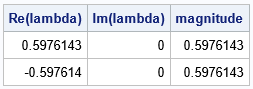
For this system of equations, the output shows that the magnitudes of the eigenvalues of the Jacobi matrix are all less than 1. Therefore, J is a contraction mapping. By the contraction mapping theorem, there is a unique fixed point, and you can find it by iteratively applying the affine transformation f(x) = c - J*x to any initial point in the plane.
The geometry of Jacobi's method
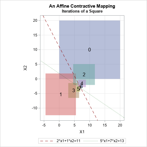
To study the contraction mapping, it is useful to visualize how the mapping transforms a rectangle in the plane. The graph to the right shows the iteration of the (blue) rectangle, R, where the lower-left corner of R is (0,0,) and the upper-right corner of R is (20,20). I have also overlaid the graphs of the two linear equations in the system. The graphs are straight lines; the intersection of the lines is the solution of the system, which we are trying to find.
The image of the square under the affine transformation is a (red) rectangle labeled with a '1'. The second image is a (green) square labeled with a '2'. Additional iterations are labeled '3', '4', and so on.
It certainly looks like the area of each rectangle is getting smaller, as you would expect from a contraction mapping. For any point p and q in the plane, you can write down the squared Euclidean distance from p to q and from f(p) to f(q) to convince yourself that, yes, the affine transformation shrinks the distance between any two points.
Geometrically, you can think of this graph as illustrating the distance between two points p=(0,0) and q=(20,20), which are the corners of the initial square. The distance between these points is the length of the diagonal of the square. Under iteration of the affine mapping, the distance between the images shrinks. The distance between the images is the length of the diagonal for each rectangle in the image.
Summary
In summary:
- Jacobi's method works by converting a system of linear equations into a fixed-point problem. For a diagonally dominant matrix (A) the associated Jacobi matrix (J) has eigenvalues that are less than 1 in magnitude. That implies that the Jacobi iteration is a contraction mapping, and by the contraction mapping theorem, there is a unique fixed point. Furthermore, the Jacobi iteration converges to that fixed point for any initial guess.
- The intuition behind Jacobi's method is that the iteration of the affine mapping f(x) = c - J*x is a contraction mapping, so any initial guess converges to a fixed point. xsoln. If xsoln = c - J*xsoln then, by construction, xsoln is a solution to the original system A*xsoln = b.
- The geometry of Jacobi's method is shown by the graph in the previous section. Iterations of the affine mapping f(x) = c - J*x map all points closer and closer to the solution of the system. The graph also shows that the mapping is a contraction.
