In a first course in numerical analysis, students often encounter a simple iterative method for solving a linear system of equations, known as Jacobi's method (or Jacobi's iterative method). Although Jacobi's method is not used much in practice, it is introduced because it is easy to explain, easy to implement, and it serves as a first example of solving a system of equations by a series of successive approximations starting from an initial guess.
A system of linear equations can be represented as a matrix equation A*x = b. The main reason that Jacobi's method is not used in practice is because Jacobi's method only converges for a special class of matrices, A. You can describe the exact mathematical requirements in terms of the eigenvalues of an associated matrix, but in introductory courses, students are told that the convergence is assured if A is diagonally dominant. This means that for each row of A, the magnitude of the diagonal element (|A[i,i]|) is larger than the sum of the magnitudes of all the other elements in that row. Intuitively, the matrix A is "close to" a diagonal matrix. We also require that no diagonal element of A is zero.
Jacobi's method is an excellent programming exercise for learning a matrix-vector language such as SAS/IML or MATLAB. This article demonstrates Jacobi's method in the SAS IML Language.
The steps of Jacobi's method
You can find the steps of Jacobi's method in textbooks and online sources, such as this reference page from the MAA. The main steps are:
- Write A = D + M, where D is a diagonal matrix and M has zeros along the main diagonal.
- The matrix equation is therefore (D+M)*x = b, which can be rewritten as D*x = b - M*x.
- If D is invertible, the equation becomes
x = D-1b - (D-1M)*x. Jacobi's method assumes that you can solve this fixed-point problem by
an iterative method:
xk+1 = D-1b - (D-1M)*xk+1
by starting with any initial guess, x0. The inverse of a diagonal matrix is trivial: If D[i,i] ≠ 0 is the i_th diagonal element of D, then 1/D[i,i] is the i_th diagonal element of the inverse of D.
The following SAS IML program implements Jacobi's method for the 2x2 example used in the Wikipedia article. First, let's use the built-in SOLVE function to solve for the vector x that exactly solves the linear system A*X = b:
/* the Jacobian method: Example from Wikipedia article https://en.wikipedia.org/wiki/Jacobi_method */ proc iml; /* define the linear system of coefficients (A) and RHS (b) */ A = {2 1, 5 7}; b = {11, 13}; xSoln = solve(A, b); /* direct method */ print xSoln ; |

The SOLVE function uses a matrix decomposition (called the LU factorization) to solve the linear system. This is an example of a "direct method" for solving the linear system. In contrast, the Jacobi method is an iterative solution. With each iteration, the approximation gets closer to the true solution (assuming that the method converges). The following SAS IML statements implement Jacobi's method. I use two techniques for efficiency:
- The equation xk+1 = D-1b - (D-1M)*xk+1 is rewritten as xk+1 = c - J*xk+1, where c = D-1b and J = D-1M. The matrix J is known as Jacobi's matrix.
- The inverse of D is never computed. It is more efficient to use elementwise division than to multiply with an inverse diagonal matrix.
- In terms of the original matrix of coefficients, J[i,j] = -A[i,j]/A[i,i] for i ≠ j, and J[i,i]=0.
In practice, you only need two vectors (often named xPrev and xNext) to implement the algorithm, but I will store the complete iteration history in a matrix so that we can graph the iteration from the initial guess to the approximate solution:
maxIters = 100; /* maximum number of iterations */ x = j(nrow(A), maxIters, .); /* store iteration history and error history for analysis */ errHist = j(maxIters, 1, .); /* decompose A = D + M where D=diag(A) is diagonal and diag(M)=0 */ D = diag(A); M = A - D; x0 = j(nrow(b), 1, 0); /* use any initial guess. Here, use the zero vector */ x[,1] = x0; /* so that we can plot the iterations, save the trajectory */ delta = 1E-3; /* convergence criterion: stop when ||A*x - b|| < delta */ err = norm(A*x[,1] - b); errHist[1] = err; /* OPTIONAL: remember the error at each step */ /* The iteration is x[,k+1] = (b - M*x[,k]) / d; or x[,k+1] = c - J*x[,k]; where c = b/d and J = M/d. */ d = vecdiag(D); /* let d be a column vector instead of a matrix */ c = b/d; J = M/d; do k = 1 to maxIters-1 until(err < delta); x[,k+1] = c - J*x[,k]; err = norm(A*x[,k+1] - b); errHist[k+1] = err; /* OPTIONAL: remember the error at each step */ end; print k err[L='error'], (x[,k])[L='x Approx']; /* save iteration history for plotting */ varNames = 'x1':(cats('x',char(ncol(A)))); /* {'x1' 'x2' ... 'xp'} */ IterHist = T(x) || errHist || T(0:maxIters-1); varNames = varNames || {'Error' 'Iter'}; create IterHist from IterHist[c=varNames]; append from IterHist; close; QUIT; |
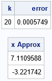
The Jacobi iteration requires only matrix multiplication and vector addition. The output shows that the method used 20 iterations to obtain an approximate solution, which agree with the exact solution to three decimals. After 20 iterations, the error in the prediction is less than the convergence criterion, which is 0.001.
Plotting the iteration history
So that we can better understand the convergence of Jacobi's method, let's plot the iteration history and the error at each step. The following DATA step adds a label for the first 10 iterations. The call to PROC SGPLOT creates a graph that visualizes how the partial solutions converge to the true solution at (7.1, -3.2).
data Jacobi; length label $2; set IterHist EVec; label = ' '; if Iter < 10 then /* show only first 10 labels */ label = putn(Iter, "2."); run; title "Iteration History"; title2 "x0 = 0"; proc sgplot data=Jacobi noautolegend; series x=x1 y=x2 / markers datalabel=label datalabelattrs=(size=12); xaxis grid; yaxis grid; run; |
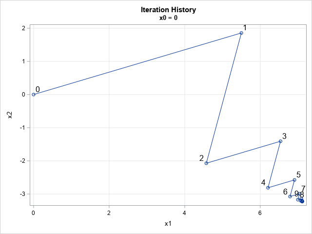
The solution to the linear system is in the lower right corner of the graph. The initial guess (marked as '0') is the point (0,0). Each iteration of Jacobi's method is marked by the iteration number: 1, 2, 3, ..., 9. For convenience, the partial solutions are connected by line segments. After nine iterations, the subsequent iterations are indistinguishable at this scale.
In a similar way, you can graph the size of the error at each iteration:
title "Error ||A*x[k] - b||"; title2 "x0 = 0"; proc sgplot data=IterHist; where not missing(error); series x=Iter y=Error; xaxis grid; yaxis grid; run; |
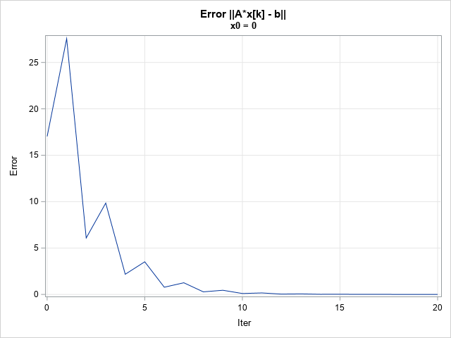
The graph shows that the error decreases rapidly for the first 10 iterations. If you were to zoom in on the next 10 iterations, you would see a similar behavior. After 20 iterations, the error is less than 0.001.
A second example
Now that we have demonstrated the basic ideas on a 2 x 2 example, how can we modify the program to handle larger systems of equations? Would you believe that you don't need to change a single line of SAS IML code? When you use matrix expressions for programming, the same statements often solve arbitrarily large matrix problems. That is the beauty and utility of representing problems in terms of matrix computations.
To demonstrate a larger example, go the beginning of the SAS IML program and replace the definitions of the A matrix and the b vector by using the following statements:
/* the matrix A is a diagonally dominant Toeplitz matrix */ A = {50 2 1 3 -1 5, 2 50 2 1 3 -1, 1 2 50 2 1 3, 3 1 2 50 2 1, -1 3 1 2 50 2, 5 -1 3 1 2 50 }; b = {94, -37, 146, 59, -4, -79}; |
You can then run the entire program without any additional modification. In only seven iterations, the program estimates the solution to be very close to the exact solution, which is {2, -1, 3, 1, 0, -2}. The graphs show the convergence of the iterations (in the first two coordinates) and the size of the error at each iteration.
Summary
This article shows how to implement Jacobi's iterative method for solving a linear system of equations. Jacobi's method uses only matrix multiplication to iterate an initial guess to a solution. Although not often used in practice, Jacobi's method provides a nice example of using matrix-vector expressions to implement an iterative multivariate algorithm.

1 Comment
Pingback: The geometry of Jacobi's method - The DO Loop