A previous article discusses the birthday problem and its generalizations. The classic birthday problem asks, "In a room that contains N people, what is the probability that two or more people share a birthday?" The probability is much higher than you might think. For example, in a room that contains N=23 people, the chance is greater than 50% that two or more share a birthday. Because there are 365 possible birthdays, many people are surprised by this result.
The birthday problem has natural inverse formulation: For a specified probability, how large must N be before the probability exceeds the specified value? For example, the inverse formulation specifies p = 0.5, and asks how many people must be in a room before the probability exceeds p. The answer is N = 23.
Mathematically, the usual birthday problem is an example of evaluating a cumulative distribution function (CDF). The inverse formulation can be solved by computing quantiles of the distribution. This article implements the CDF and the quantile function for the generalized birthday distribution as functions in the SAS IML language. For completeness, I also provide the PDF of the distribution, and a function that returns random values from the distribution. You can download the functions from GitHub.
Approximating the quantile function
A previous article uses a formula in a paper by Diaconis and Mosteller (2002) to approximate the CDF function, which depends on N and other parameters (C, the number of categories, and D, the number of shared values). For a specified probability, you can invert the formula by solving for N. However, you will get a decimal number such as 22.9. Because N must be an integer, you need to round the answer.
Furthermore, the "birthday distribution" is a discrete probability distribution, so the quantiles are defined in terms of an inequality: For a specified probability p, return smallest integer, N, such that CDF(N) ≥ p. Thus, after obtaining an estimate of N, you might need to increment it or decrement it until you obtain the correct value.
This method is implemented in the QuantileBirthday function, which you can download from GitHub. The function is modeled after the qbirthday function in R, which uses the same Diaconis-Mosteller formulas.
Let's run the QuantileBirthday function on a few examples:
- First, the classic example: how many people must you consider before the probability of a shared birthday exceeds 50%? (Answer: 23)
- A generalization: how many people must you consider before the probability of three people sharing a birthday exceeds 50%? (Answer: 88)
- How many people before the probability of four people sharing a birthday exceeds 50%? (Answer: 187)
/* first, download the functions from GitHub and STORE them https://github.com/sascommunities/the-do-loop-blog/blob/master/birthday-problem/genbirthday.sas Run that file or %INCLUDE it before running the following statements, which LOAD the functions. */ proc iml; load module=(expm1 CDFBirthday PDFBirthday QuantileBirthday RandBirthday); *classical birthday problem; N2 = QuantileBirthday(0.5); /* find N s.t. Pr(2 BDays) >= 0.5 */ N3 = QuantileBirthday(0.5, 365, 3); /* find N s.t. Pr(3 BDays) >= 0.5 */ N4 = QuantileBirthday(0.5, 365, 4); /* find N s.t. Pr(4 BDays) >= 0.5 */ print N2 N3 N4; |

The QuantileBirthday function produces the correct results in each case.
You can also use the QuantileBirthday function to compute an example in Diaconis and Mosteller (2002, p. 858). They tell the story of a mother, father, and child who were all born on the same day of the month. (For example, they could be born on the 16th of December, the 16th of April, and the 16th of October.) Diaconis and Mosteller compute how large a group must be before the chances of observing this situation exceeds 50%. Instead of C=365 birthdays, this problem uses C=30 equally likely days in a month.
*Three BDays are on the 16th, but different months; *What size group gives equal prob of this occurence?; N3_30 = QuantileBirthday(0.5, 30, 3); *assumes 30 days in month; print N3_30; |

The table shows that you should expect this coincidence in a family that has 18 or more people.
A graph of the quantile function
You can graph the quantile function by evaluating it on a coarse grid of values in the interval (0, 1). The following graph shows the quantile function for the classic birthday problem (365 equally probable birthdays, looking for a birthday that is shared by two or more people):
prob = do(0.05, 0.95, 0.0025); Q = j(1, ncol(prob)); do i = 1 to ncol(prob); Q[i] = QuantileBirthday(prob[i], 365, 2); *default C=365, num dups D=2; end; title "Quantile Function for Classic Birthday Problem"; title2 "Assume 365 Equally Likely Birthdays"; call series(prob, Q) grid={x y} xvalues=do(0.1,0.9,0.1) yvalues=do(5,50,5) label={"Prob(Matching)" "Number of People (N)"}; |
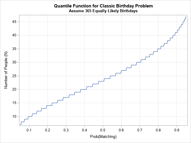
Notice that the graph is a step function, as it is for every quantile function of a discrete distribution. For any probability, p, the graph shows the size of a group in which the probability of a shared birthday exceeds p. By changing the value of the third parameter (D, the number of people who must shared a birthday), you can make similar graphs for three shared birthdays or for four shared birthdays. By changing the second parameter (C, the number of unique, equally likely values for each person), you can create similar graphs for a shared birth month (C=12), a shared day-of-the-month (C=30), and so forth.
The PDF function and random value generation
I think the CDF and quantile functions are the most important functions for the generalized birthday problem. However, for completeness, I have implemented functions that computes the PDF and that generate random variates.
Technically, the PDF is called a probability mass function (PMF) because the distribution is discrete. It should be plotted by using a bar chart or a needle plot. However, when there are many categories (large values of C), it is common to plot the PMF as if it were continuous. (This is also common for the binomial distribution, the Poisson distribution, and other discrete distributions that can produce a large range of integer values.) For example, the following statements create the PMF for the classic birthday problem and plot it as if it were a continuous density:
N = T(1:60); PDF = j(nrow(N), 1); do i = 1 to nrow(N); PDF[i] = PDFBirthday(N[i], 365, 2); * C=365, D=2; end; title "Probability Density for Two Shared Birthdays"; title2 "Assume 365 Equally Likely Days"; call series(N, PDF) grid={x y} label={"Number of People (N)" "Density"}; |
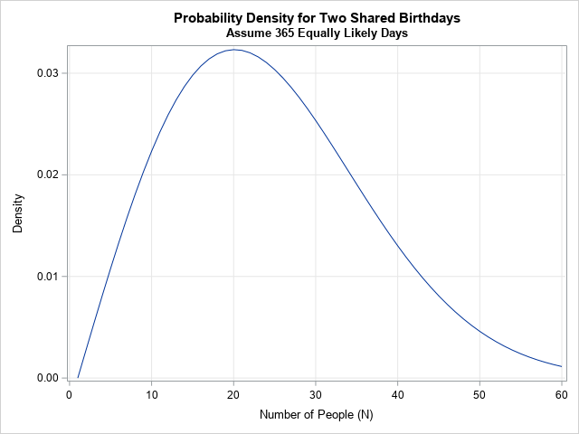
The graph of the PDF shows that N=20 is the most probable value for a group of size N to have a shared birthday, followed closely by N=19 and N=21.
You can also generate random variates for the birthday problem by using the RandBirthday function. For example, if you ask for five random variates for the classic birthday problem, you will get five random sizes of rooms in which two individuals share a birthday, as follows:
* test the RandBirthday function; call randseed(54321); Sizes = RandBirthday(5); print Sizes; |
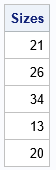
In this instance, we assume that we gather random groups of people until there is a shared birthday within the group. From theory, we know that, on average, you expect a room with N=23 people to contain a matching birthday. However, in reality you might get a match in a group of N=13 people, or you might have to gather N=34 (or more) people before there is a match. The output shows five sizes of groups that have a matching birthday. If you generate many groups, the histogram of the random values looks like the graph of the PDF function.
Summary
The classic birthday problem has an exact CDF when you want D=2 shared birthdays in a group of size N. The generalized birthday problem has an approximate solution when D > 2. For both cases, you can invert the (exact or approximate) formula for the CDF to obtain the quantile function for the birthday problem. You can also take first-order differences to obtain a PDF function, and you can use the inverse-CDF method to generate random variates. You can download the SAS IML functions for these computations from GitHub.
