Use design matrices to analyze subgroups in SAS IML

A previous article shows ways to perform efficient BY-group processing in the SAS IML language. BY-group processing is a SAS-ism for what other languages call group processing or subgroup processing. The main idea is that the data set contains several discrete variables such as sex, race, education level, and so on. You want to perform the same analysis on each subgroup of the data, such as analyze the mean income of white males, black males, white women, black women, and so forth.

I have previously written about the one-way analysis of groups and compared the performance of the UNIQUE-LOC method and the UNIQUEBY method. The UNIQUE-LOC method is an intuitive way to structure the analysis of subgroups. You loop over the unique values of a grouping variable, extract the observations that correspond to each level, and analyze the levels.

Unfortunately, if you have two grouping variables, the UNIQUE-LOC technique is more complicated to program. You need to use two loops. For each iteration of the first loop, you must subset the data. You then analyze subgroups of the subgroups inside a second loop. For three grouping variables, the UNIQUE-LOC trick requires programming three nested loops.

There is an easier way to program the analysis of subsets. I call it the design-matrix method because it constructs design matrices for each classification variable and then uses the horizontal direct product operator to obtain the design matrix for the interaction effect between the classification variables. This article provides the details. In this article, "the design matrix" always refers to the so-called "GLM parameterization" in which each column of the matrix is a binary indicator variable.

The horizontal direct product between design matrices

The horizontal direct product between matrices A and B is formed by the elementwise multiplication of their columns. The operation is most often used to form interactions between dummy variables for two categorical variables. If A is the design matrix for the categorical variable C1, and B is the design matrix for the categorical variable C2, then HDIR(A,B) is the design matrix for the interaction effect C1*C2.

Let's look at a small example. The Sex variable has values 'Male' and 'Female'. The Race variable has values 'White', 'Black', and 'Asian'. The following SAS IML statements create a design matrix for each variable. The HDIR function computes the horizontal direct product, which is the design matrix for the interaction term Sex*Race:

/* demonstrate the design-matrix technique on a small data set */
data Have;
length Sex $6 Race $8;
input Sex Race;
datalines;
Male   Black
Male   White
Female Asian
Female White
Female White
Female Asian
Male   White
Male   Asian
Male   Black
;
 
proc iml;
use Have;
   read all var {"Sex" "Race"};
close;
D1 = design(Sex);
D2 = design(Race);
print D1[c={"Female" "Male"}], D2[c={"Asian" "Black" "White"}];

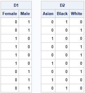
The D1 design matrix encodes the values of the character variable, Sex. The D2 design matrix encodes the values of the Race variable. From D1, you can read off the sex of each observation. The first two observation are male, the next four are female, and so forth. Similarly, from D2, you can read off the race of each observation: Asian, black, or white.

The horizontal direct product of D1 and D2 combines the information into a single matrix that has six columns. The first three columns encode the race for females; the last three columns encode the race for males.

HDir  = hdir(D1, D2);
labl = {"F-Asian" "F-Black" "F-White" "M-Asian" "M-Black" "M-White"};
print HDir[c=labl];

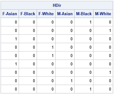
In this table, the value 1 appears only once in each row. The column in which the 1 appears tells you the sex and race of the corresponding observation. Furthermore, the sum of the columns tells you how many of each joint level are in the data. For this small sample, there are no black females, as you can see by noting that the second column does not have any 1s. You can see that there are two white females by looking at the third column.

Two-way tabulation: An application of the design-matrix technique

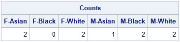
The first application of the design-matrix technique is to obtain the counts for each joint level of the two (or more!) grouping variables. As mentioned in the previous section, the sum of each column tells you the number of observations who are female-Asian, female-black, ..., male-white:

/* 2-D tabulation of counts */ 
Counts = HDir[+,];
print Counts[c=labl];

A general two-way analysis technique

The design-matrix method provides a general technique to perform a two-way analysis of the subgroups that are defined by the joint levels of two categorical variables. Suppose the first categorical variable has k₁ levels and the second variable has k₂ levels. If H is the direct-product matrix of the design matrices for the two categorical variables, it has (k₁ x k₂) columns, although some of the columns might contain all 0s. By looping over the columns of the direct-product matrix, you can quickly identify the observations (if any) in each subgroup.

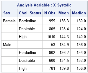
To demonstrate this method, the following SAS DATA set contains observations from the Sashelp.Heart data set, which contains data about patients in a clinical study. To make the method easier to understand, I rename the Sex and Chol_Status categorical variables to be G1 and G2, respectively. I rename the systolic (blood pressure) variable to be X. The goal of the analysis is to compute the size, mean, and median statistics for X for each joint level of G1 and G2. To make the problem more interesting, I exclude one of the joint levels, which will cause the direct-product matrix to have a column of 0s. The following SAS statements create the data set and use the CLASS statement in PROC MEANS to obtain the statistics for each subgroup. Because I want to include patients for which the cholesterol status is unknown, I use the MISSING option on the PROC MEANS statement:

data Heart;
set sashelp.Heart(where=( ^(Sex='Female' & Chol_Status=' ') ));
G1 = Sex;
G2 = Chol_Status;
X = Systolic;
keep G1 G2 X;
label G1='Sex' G2='Chol_Status' X='Systolic';
run;
 
proc means data=Heart mean median missing ndec=1;
   class G1 G2;
   var X;
run;

You can use the design-matrix technique to obtain the same statistics by writing a single loop in SAS IML that iterates over the columns of the direct product of the design matrices of G1 and G2:

/* Goal: analyze each level of (G1, G2) */
proc iml;
use Heart;
   read all var {"G1" "G2" "X"};
close;
 
/* 1. Get the levels of the categorical variables */
uG1 = unique(G1);              /* levels for G1 */
uG2 = unique(G2);              /* levels for G2 */
uAll = ExpandGrid( uG1, uG2);  /* joint levels (some might be empty) */
SubGroupNames = rowcatc(uAll[,1] + '_' + uAll[,2]); /* create labels */
*print SubGroupNames;
 
/* 2. Create the design matrices and the horizontal direct product */
D1 = design(G1);               /* design matrix for G1 */
D2 = design(G2);               /* design matrix for G2 */
D  = hdir(D1, D2);             /* horizontal direct product */
*print (D1[1:10,])[c=uG1], (D2[1:10,])[c=uG2], (D[1:10,])[c=SubGroupNames];
 
/* 3. perform an analysis of subgroups */
stats = j(nrow(uAll), 3, .);   /* allocate result matrix: N, Mean, and Median */
stats[,1] = 0;                 /* counts default to 0 */
do i = 1 to ncol(D);
   idx = loc(D[,i]);               /* obs where D[,i]=1 define subgroup */
   if ncol(idx) > 0 then do;
      subset = X[idx,];            /* extract the obs */
      stats[i,1] = ncol(idx);      /* N for subgroup */
      stats[i,2] = mean(subset);   /* mean for subgroup */
      stats[i,3] = median(subset); /* median for subgroup */
   end;
end;
print stats[r=SubGroupNames c={'N Obs' 'Mean' 'Median'} F=Best5.];

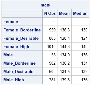
The output from the SAS IML program is equivalent to the output from PROC MEANS. The IML output includes the "empty group" of females for which the cholesterol status is missing. Of course, the power of this technique is that you can use this method to perform subgroup analyses that are not supported by any other SAS procedure.

The program shows how to perform a two-way analysis of subgroups. The program for three or more subgroups is equally simple: let D1, D2, ..., Dm be the design matrices for the categorical variables and define D = HDIR(D1, D2, ..., Dm). Then loop over the columns of D as shown above. In other words, the code for the design-matrix technique supports 2, 3, or more categorical variables.

Drawbacks of the design-matrix technique

Of course, there is no such thing as a free lunch. Whereas the UNIQUE-LOC method requires very little memory, the design-matrix method requires more memory. If there are N observations and the m categorical variables have k1, k2, ..., k_m levels, then the direct product matrix is an (N x (k1 k2 ... k_m)) matrix. Accordingly, the design-matrix technique is best used on medium-sized data sets and with categorical variables that have a small number of levels.

You can extend the UNIQUEBY method to support multiple categorical variables. The UNIQUEBY technique requires a much smaller memory footprint. However, the UNIQUEBY method requires that the data are sorted whereas the design-matrix method does not.

Summary

The UNIQUE-LOC method is an easy and intuitive method of performing a subgroup analysis for levels of a single categorical variable. However, the natural generalization of the method to multiple categorical variables requires that you write nested loops and keep track of subgroups of subgroups. In contrast, the design-matrix method uses only a single loop to iterate over the columns of a matrix that is the direct product of the design matrix for arbitrarily many categorical variables. This article demonstrates how to use the design-matrix method to perform a subgroup analysis.

Blogs